The Foot Of Slope (FOS)
Introduction
Some of the lines used to define the outer limit of the continental shelf are based on a line called the Foot Of Slope (FOS). UNCLOS article 76 defines FOS as follows: "In the absence of evidence to the contrary, the foot of the continental slope shall be determined as the point of maximum change in the gradient at its base."
Geocap has two methods to visualize the change of gradient. One is to map a surface with its change of gradient in the gradient direction. Another method is to analyze the gradient along a bathymetric profile.
In this section:
Mapping the change in gradient
The schema seabed surface by default has two commands called Map derivative and Gradient Band Analysis, which are used for mapping a surfaces with their change in gradient.
Map derivative
Using the Map derivative command, you may map a surface with its gradient size, the gradient direction, or the change of gradient in the gradient direction. If you select more than one display, all the displays will be showed in the display window at the same time. You can select which ever display you want to see by checking on and of the check boxes to the left of the actor items in the project.
You can display the data using two display methods. Using scalar values, you will create one gradient value pr grid node in the display data set. When using texture mapping, you will display a scalar value for each grid node in the original data set, which may be more detailed than the display data set. The Texture map will therefore often give a more detailed display. You can also smoothen the input data set before the derivative calculations are performed.
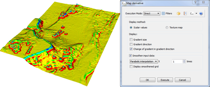
Mapping derivative menu and result
When you execute the command displaying the change of gradient in the gradient direction, you may need to adjust the color table range in order to get the information you want. Read more about adjusting map range.
Gradient Band Analysis
The Gradient Band Analysis command lets you display color bands by dividing the grid into different areas depending on the steepness of the grid. The boundaries are set in degrees and may be adjusted by to change the area between them.
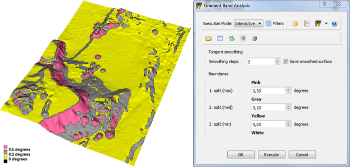
Gradient band analysis menu and result
Creating Bathymetric Profiles
Geocap can also be used to study the change of gradient along a bathymetric profile. The profile can either be loaded from a file, or digitized from a seabed surface. Single beam Bathymetry can be used as a bathymetric profile directly. Multibeam bathymetry must be gridded first. Then profiles can be extracted from the bathymetric grid.
Loading from a File
Right click a Bathymetric lines folder and select import. Use any of the import methods. Select the schema bathymetric profile for the new data set.
Digitize from Bathymetry grid
Right-click a Bathymetry grid with the schema seabed surface and select the command Generate bathymetric profile. Click start in the dialog that appears, and click on two points on the seabed surface in the 3D display window. In order to do this you have to display the seabed surface first (e.g. with the map data command.) A bathymetric profile will be created, and put in the folder named 2. Seabed/Bathymetric Profiles
Moving and Resampling an Existing Profile
Right-click a profile which has been sampled from a seabed surface, and select analyze profile. The 2D analysis window will appear. In the 3D display window, move the profile by dragging the cross section or dragging the spheres in the corners of the cross section. When you move the profile, the 2D analysis window is automatically updated. When you are satisfied with the location of the new profile, click the Save Profile As in the 2D analysis window. The new bathymetric profile will be stored in the same folder as original profile.
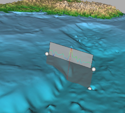
The analyze profile in 3D view
Bathymetric Profile Analysis
Geocap contains a bathymetric profile analysis tool which can be used to define the foot of slope based on the maximum change of gradient. The same tool can be used to study the gradients along a profile. The tool is opened by selecting the analyze profile command on a bathymetric profile. This will open up a panel consisting of two parts; a 2D graph display on top and the analysis workflow at the bottom.
The profile analysis panel may be in two modes; Profile mode or Analysis mode. When you open the panel it will be in Analysis mode. Once the user user starts moving the profile in the 3D display window, it will enter Profile mode. When in Profile mode, the profile you see in the dialog is not stored in the project, only temporary in the menu. The modified profile has to be stored in the project, like explained in the previous section, before an analysis can be stored with it. This is done by pressing the Save Profile As button. This will store the new profile in the same folder as the original profile, and the dialog will enter Analysis mode again.
When in Analysis mode the user may store the settings in the analysis. The new analysis will be stored as a child of the profile in the project. The command which was used to generate the analysis will be stored as a command of the analysis. If the analysis is a change of gradient analysis, a foot of slope point may also be stored as a child of the analysis in the project.
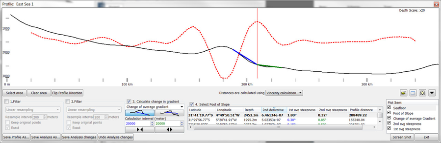
The Foot of Slope Analysis dialog
2D profile
By default, the 2D graph display window contains a black solid line representing the bathymetric profile. The red dotted line is the change of gradient, normalized to fit the window with a gradient equal to zero in the middle. The red solid vertical line is the foot of slope point.
You are able to zoom and pan into this window just as in 3D window; zoom by holding in the right button and moving the mouse. You can pan by holding in the middle button while moving the mouse. You scale the z value by scrolling with the mouse scroll butting. The depth exaggeration is displayed in the top right corner. Notice the rulers at the bottom and to the left.
By using the select area button, the user may select an area in the 2D display window using the left button on the computer mouse. The gradient analysis, or change of gradient analysis will only be preformed in this area. The area which is not selected for the computation is shaded in gray. The Clear area button clears this area.
The Flip profile direction button is used to flip the horizontal direction of the view of the profile.
Analysis workflow
The foot of slope utility workflow. The first and second filter are optional.
The analysis workflow consists of running one or two filters on the bathymetric profile, then computing the gradient or change of gradient and then selecting which foot of slope points to use.
Input
The bathymetric profile used as input is "straightened" in a coordinate system where the horizontal axis represents the distance along the profile, and the vertical axis represents the depth. The distanced along the straightened profile may be computed using a simple Euclidean distance calculations in the local coordinate system, or by using an algorithm taking the earth curvature into consideration. The computations done in the rest of this workflow uses this coordinate system.
Filters
The user has an option to use one or two filters before doing the actual computation. The following filters can be performed on the data:
- Resampling
- Spline approximation
- Douglas Peucker approximation
- Median filter
- Moving average filter
- Fourier low pass filter
Read more about these filters in: Filters and gradient algorithms.
If both filters are activated, filter one will be executed on the input data, while the second filter will use the output from the first filter as its input.
Calculation
The user can choose between four different gradient or change of gradient algorithms. The calculation is performed on the bathymetric profile, or the filtered output if one or more of the filters are activated. In order to create a foot of slope point, a change of gradient, or change of average gradient computation has to be performed.
The finite difference methods, calculate the first and second derivative by looking at changes in the profile at a very small interval. This method is very sensitive to noise; you should therefore consider smoothening the input data if you use this algorithm.
The other group of methods is the moving average steepness algorithms. These algorithms compute the average steepness at an interval to the left and right of each point on the line, and compares these two steepnesses in order to compute the change of gradient. These methods are not as sensitive to noise as the finite difference methods. Therefore, you usually do not need to smoothen the input data when using this algorithm. The algorithm will get less and less sensitive to noise in the input data as you increase the calculation interval.
Read more about these algorithms in: Filters and gradient algorithms
Selection
When a change of gradient analysis has been performed, all local maximum points from computation are sorted in a list. The user may select which maximum to use as foot of slope point by selection in the list. The list also contains the points position, the computed change of gradient, and the computed gradients used in the change of gradient calculation.
To the right you have a list of all the graphs displayed in the 2D display. You can toggle them on and of by clicking at the check boxes. You can also edit the lines appearance by right clicking the item in the list, and select "edit". An editor with various settings will appear.
Generating 60M Line from FOS Points
When you have created a foot of slope point or a foot of slope line, you can generate the foot of slope plus 60M line. Make sure the foot of slope data set has the foot of slope schema. Right clicking the dataset, and select the generate 60M line command.
This command works the same way as the other distance line commands.
The 60M line stored under 1. Maritime Lines / 60M lines in the project.
Metadata
By opening the table view for the FOS+60M line you can see which FOS dataset it was generated from. For each point on the 60M line you will see a reference to the point in the FOS dataset which contributed to that point.
For equidistant points you will see reference to the two points in the FOS dataset which contributed to that point.
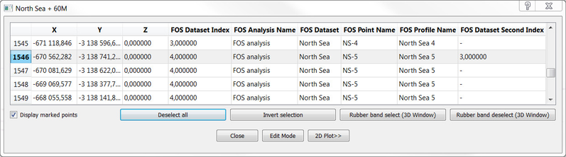
FOS+60M table view