Geocap Interface

Introduction

Geocap has a very customable interface. The user may even program a new interface and develop new functionality. The concept of commands and schemas are key elements of understanding and operating Geocap.

Exercises

Geocap project

Geocap is operated through projects. The project "holds" the data in a folder-like structure, similar to Windows "File Explorer". All datasets are "children" of either a folder or another dataset. Geocap offers different project templates, giving you a pre-defined folder structure that fits your workflow for a specific type of work.

Exercise

Open the Atlantis project

Click File > Open > Project and browse to the location of the Atlantis project.
Select the Atlantis.db file and click Open. A window similar to the one below will appear.

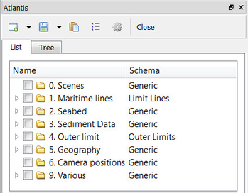
An open project

Tip

Next time you can open the project by using File > Recent Projects.

Pressing the small triangles (or '+' in older Windows versions) to the left of a folder will display the folder's contents. Datasets and folders are organized very similarly to a file tree structure. A folder can contain other folders, or datasets.

Note that there are two "modes" of the project view. Switch between these two by clicking on the tabs; List and Tree. List view sorts folder content into a separate window, while Tree view sorts everything into the tree itself..

In the next exercise we are going to explore how the Atlantis project is structured. Taking notice of how folders and datasets are organized. Datasets and folders can be cut, copied, pasted, renamed and deleted. This is performed from the popup menu which appears when right-clicking a dataset. The right click popup menu also contains commands which may be executed on the datasets. Notice the different icons of the different datasets. They correspond to the schema of the data set. The name of the schema is written in the second column.

Exercise

Explore the project folder structure

Expand the folders and observe the sub folders
Look at the right-click menus.

Display data

Exercise

Display data

Display the various datasets in the project

Locate a grid dataset (structured points or seabed) e.g. 2. Seabed/Grids/atlantis
Tick the checkbox next to the dataset to display it.
Right click the dataset again and select Zoom to Data. This will make the display window center the graphics window around the dataset.
Display some of the lines e.g. lines found under 1. Maritime Lines.

Note that by checking and unchecking the first level folder 1. Maritime Lines, or 2. Seabed all datasets displayed under this folder are shown and hidden.

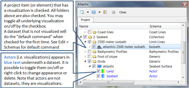
Visualizations are called actors

Exercise

Commands: In panel Help

Open the command called "Generate 200M Line" from the toolbox.
Click the icon with the question mark to open the in-panel help.
Read the information that pops up.

Navigating the graphics window

Note: Operating Geocap with a two-button mouse or using the Touch-pad is possible but not recommended. The recommendation is a three-button mouse with a wheel, see picture below.

You may use the computer mouse to move around in the display window. You do this by pressing one of the mouse buttons while the cursor is in the display window, and moving the mouse while keeping the button pressed.

Rotate - Left mouse button
Pan - Middle mouse button (or wheel) or Shift + left mouse button
Zoom - Right mouse button
Scale Z - Mouse wheel (scroll)
Spin - Ctrl + left mouse button

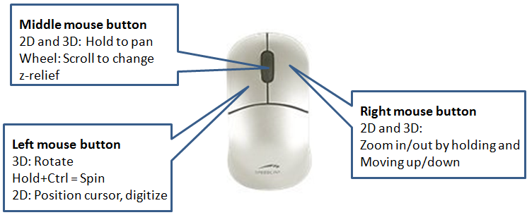
The mouse buttons

Exercise

Navigate using the mouse

Try to zoom in and out.
Try to pan.
Try to rotate the data.
Try to scroll the wheel to increase the z-scale.
Now try to examine three areas more closely my panning, zooming in closely and rotating.

Tip

Set the focal point by positioning the mouse cursor on a desired point in the display window and push the X key on the keyboard. This focal point will be the center of the display and the point of rotation.

Scrolling the mouse wheel is one way to scale depth values of the dataset. The z values can also be scaled by clicking the Actor Scale button in the toolbar and dragging the z slider.

Important Toolbar Buttons

Basic Concepts in Geocap

The interface to the UNCLOS specific features in Geocap are through the use of schemas on datasets and commands. The commands can be found in the Toolbox to the right in the Geocap interface or at the top of the menu which appear when you right click a dataset. Which commands are displayed in the right click menu depend on the schema of the dataset. A Base Line will contain commands appropriate for the Base Line schema, while a Bathymetric Profile will contain different commands.

Schemas

Geocap uses schemas to classify a dataset. The Shelf Module contains several schemas. Some of the schemas used in the Shelf Module are coast line, base line, limit line, seabed, sediment thickness. You can define the schema of a dataset in the project by right clicking it, and selecting set schema in the pop-up menu. The choice of a dataset´s schema controls which commands you see in the pop-up menu when you right click the dataset. You may create your own schemas as well as edit existing schemas by selecting schemas under edit in the main menu. You can also edit the commands associated with the schemas.

Commands

Commands are operations which can be performed on a dataset. Commands can for example be used to display a dataset in the display window, or to generate new datasets. You can even create your own scripted commands to cater to your specific needs. You execute a command by right clicking the dataset or folder you want to run it on, and then selecting the relevant command in the pop-up menu. You can give different parameters to a command in the command editor. These parameters are stored with the command and used during execution.

Commands can be stored in three categories:

Item commands
Schema commands
Shared commands.

You will find the commands sorted into the different categories in the Toolbox (see illustration below) or on the right-click menu of a dataset or a folder. Commands are also put together in sequence in Workflows to perform visualizations or data operations, see chapter S.

All commands have a front end panel, and most of them have settings that may be customized.

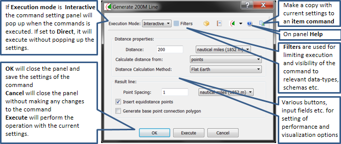
An example of a command front end panel

Item Commands

A command can be stored at the level of a dataset or a folder. This is called an item command. This command is unique to this dataset or folder, it "belongs" to that dataset. You can see these commands on the top of the Toolbox or in a sub menu when you right-click a dataset and select Item commands. Most items in the project do not contain any item commands by default.

Exercise

Create an item command

Go to 1. Maritime lines / 60M lines and select one of the datasets.
In the Toolbox right click Display.
Set Line Width to 4.
Check User defined Color and set the color to white.
Click the icon in the upper right corner of the menu and observe that the command appears in the Toolbox under Item Commands.
Click Cancel (the settings will not be saved for the schema command).
Right click the Display command under Item Commands and select Rename.
Rename it to Display in white and click OK.
Select the different lines in 1. Maritime lines / 60M lines and observe that the new Display in white command is only available for the one dataset.

Schema Commands

A command stored at a schema level is called a schema command. All datasets or folders using the same schema share these commands, which also means that editing these commands will affect all the datasets using this schema. The schema commands of a dataset are listed on the top of the right-click menu.

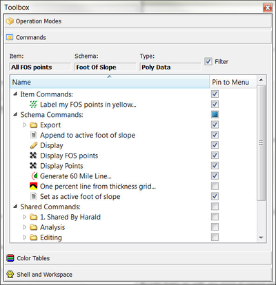
The Geocap Toolbox. Note that the Filter is checked, meaning that commands not specifically relevant are invisible. Untick the filter to show all commands.

Exercise

Get familiar with schema commands

Right click the different datasets in the project, and see how the right click menu changes from schema to schema.

Default command

The default command is the command that is executed when you tick the box next to a dataset in the project. By default a dataset will have one of the schema commands as a default command. This can however be changed.

Exercise

Change the default display for seabed surfaces

The seabed surfaces has a default command "Map sea" or something similar.

Click on the Seabed datasets in the 2.Seabed / Grids folder.
In the Toolbox right-click another command (i.e LOD Grid Display) and select Set as default command
Tick the checkbox next to the Seabed dataset and notice that the new command is executed.

Shared Commands

Shared Commands are commands which are shared with all datasets and folders. The shared commands are listed in the Toolbox under Shared commands. If you cannot see the Toolbox, it can be opened from View on the main menu.

All commands have a command editor where you may change the properties, thus affecting the way it is executed.

Exercise

Create a new command for custom display of limit lines.

Click on one of the datasets with the limit line schema inside the 1. Maritime lines folder
Right click the Display command under Schema commands in the Toolbox and select Copy
Right click Schema commands in the Toolbox, select Paste and observe that a copy of the selected command called Display-1 will appear in the schema command list.
Right click the new command in the command list, and select Rename
Name the command Display Thick Yellow
Right click the command and select Edit. The command editor for the selected command will appear
Set Line width to 6
Check the User defined color box and click the Palette button.
Select a yellow color and click OK
Click OK to close the Display command editor
Right click the same data set, and observe that our new command is present in the right click menu. This is because the Pin to Menu check box next to the Display Thick Yellow command in the Toolbox is checked.
Un-check the Pin to Menu check box next to the Display Thick Yellow command in the Toolbox.
Right click the same data set again, and observe that our new command is not present in the right click menu.
Execute the command by double clicking Display Thick Yellow in the Toolbox. Observe that the line is displayed in yellow.
Check the Pin to Menu check box next to the Display Thick Yellow command in the Toolbox again. Now right click a different dataset with the same schema (limit line) and observe that the new command can be executed on this right click menu as well.

Tip

The Pin to Menu check box lets you decide which commands should be available in the right click menu, so it is easy to keep organized. Try to experiment with this option to manipulate the right click menu.

The Sticky Surface

Geocap has a concept where any surface can be set to be sticky. When a surface is sticky, data like points, lines or images may be displayed onto that surface. This is mainly done by re-sampling lines and displaying them a little bit above the sticky surface.

When a surface is activated (or set) as a sticky surface, it is copied to workspace (visualized in the toolbox) under the name sticky_surface. If this dataset is removed from workspace, there is no sticky surface anymore.

Exercise

Display onto the Sticky Surface

Right-click on a Seabed surface dataset and select Set as sticky surface
Select a line, e.g. Atlantis > 1. Maritime lines > 200M lines > atlantis + 200M in your project.
In the Toolbox under Commands > Schema commands right-click and Edit on the Display command.
Check the Glue to Sticky Surface and press Execute to do a line display.
Uncheck the Glue to Sticky Surface and press Execute again and observe the difference.

Warning

Note that points and lines displayed onto a sticky surface are displayed without their original z-values, and this may not be what you intend to do when displaying a foot of slope point or a bathymetric line. Keep that in mind.

Keyboard shortcuts

Geocap has several keyboard shortcuts or hotkeys. Go Help > Keyboard shortcuts to bring up a list.

A selection of the most important keyboard shortcuts:

Key	Explanation	Key	Explanation
o	Toggle color code for last used map command on/off.	+	Zoom in.
s	Turn graphics into surface mode.	-	Zoom out.
v	Value of height/depth (z coordinate) from graphics.	2	Toggle graphics to 2d mode.
w	Turn graphics into wire mode.	3	Toggle graphics to 3d mode.
x	Setting the focal point. The graphics will rotate around this point.	3	Toggle stereo view on/off when stereo is activated.
y	Cursor point is set at the surface of the graphical element.	z	Zoom by drawing a rubber band with left button on the mouse.
j	Snap to any point on a displayed line.

When using j or y to snap to lines or surfaces, Geocap will report what you have snapped to in the lower left corner.

Exercise

Keyboard shortcuts

Visualize a seabed surface and test all the above mentioned keyboard shortcuts.