Maritime Zones plugin

The Maritime Zones calculation wizard

A short history of the Maritime Zones plugin

The Maritime Zones plugin was developed in close cooperation with Geoscience Australia. The project was started in early 2013. The expert knowledge provided by Geoscience Australia regarding maritime zones in general and straight baselines in particular has been key in the design and development of this important extension to the Geocap Shelf module. 

Prerequisites

The requirements for using the Maritime Zones plugin are:

• The Datalink for ArcGIS plugin. This itself is a separate licensed feature that requires an ArcGIS Desktop license to be available on your machine
• Geocap 6.5 32 bit (neither the Maritime Zones plugin or the Datalink for ArcGIS plugin is available in the 64 bit versions of Geocap)
• The Shelf package

Please contact Geocap sales for information on how to obtain these components.

Usage

How to load the Maritime Zones plugin

1. Click Tools, then Options
2. In the Options dialog select the Plugins page
3. Check the Datalink for ArcGIS and Maritime Zones plugins
4. In the ArcGIS Version field choose the version of ArcGIS that is installed on your machine.
5. Click the OK button to close the dialog
6. The checked plugins will be loaded

Calculating maritime zones

This section desribes how to calculate maritime zones from an ArcGIS feature class containing the base line.

To calculate maritime zones:

1. Click the '+' button on the ArcGIS toolbar and add the base line feature class to your map in the table of contents 
2. Right-click the resulting base line feature layer in the Table of Contents, then click Calculate Maritime Zones. The calculation wizard will appear.
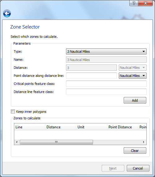
3. The first page in the wizard contains the paremeter setup for each distance:
   1. Enter the corresponding parameters for the given distance, including the name of the output feature classes that will contain the distance line and critical points.
   2. Click Add to add the distance to the pool of distances that will be calculated
   3. When all distances are added, click Next 
4. Page two in the wizard gives you the option of calculating straight baselines. If you wish to include straight baseline calculation:
   1. Check the entry The baseline feature class contains straight baselines
   2. In the field Baseline type column select the column that contains the straight baseline attribute
   3. In the Attribute field enter the attribute value that denotes a straight baseline, or click Browse to select from the list of which unique attribute values that are present in the straight baseline column
5. In the field Temporary working directory you may choose to override your systems default temporary directory that will be used during the calculation
6. Click Next to see the final summary page. 
7. If you are satisfied with the values entered in the wizard click Finish to begin the calculation
8. For each maritime zone that is calculated the resulting feature layers containing the critical points and distance lines will be added to the map in the Table of Contents

The distance calculation algorithm

This section describes in detail the algorithm used in the calculation of maritime zones, including straight baseline calculation.

Geocap can calculate geodetic correct distance lines from baselines. The distance lines can be based on normal baselines, straight baselines, or a combination of normal and straight baselines.

All distances are calculated using the  Vincenty algorithm.

This technical documentation will give you an understanding of how distance lines are generated in Geocap. In the real implementation, optimizations are done in order to handle large amounts of data, and large areas. These optimizations are not discussed here.

Algorithmic overview

The input to the algorithm is a base line dataset, which may be a combination of straight and normal base lines.

1. The Straight baselines are resampled.
2. A “distance grid” is calculated from the baseline.
3. A grid contouring is performed on the distance grid, with the contour value set to the desired distance.
4. Each point on the limit line is examined, and position is set accurately.
5. The limit line is checked for topology errors.
6. Equidistant points are inserted.
7. The distance line is resampled with the desired limit line point spacing.
8. Each point on the limit line is examined, and position is set accurately.

Algorithmic  details

1. Straight base line resampling

Straight baselines are resampled by inserting new points on the geodesic between the end points of the straight baseline, with a sample interval sufficient for the next steps in this distance calculation.

2. & 3. Distance grid and contouring

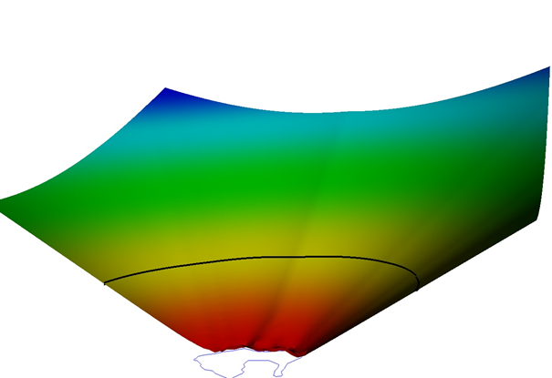
Figure 1: A distance grid with a contour displayed in 3D. The color represents the distance from the baseline. The black line is a contour on the distance grid.

A distance grid is created. The value of each grid node is set to the distance from the grid node center to the nearest baseline point. The grid spacing is set to a value smaller the desired point spacing of the distance line. The grid extent is set large enough to cover all distance lines.

The grid is contoured at the desired distance value.

4. Adjusting limit line points

Each point on the limit line is examined. For each limit line point, the nearest baseline point is located and the line point position is set accurately. The baseline point id is also stored for later use.

• If the nearest point is a normal baseline point, the distance point position is set accurately with the desired distance from the normal base point.
• If the nearest point is one of the resampled straight baseline points from step 1. The resampled points are ignored, and a new position is calculated from the geodesic between the end points of the straight baseline.

5. The limit line is checked for topology error

The limit line may at this point contain some topology errors due to the contouring in step 3. The contouring algorithm may do wrong connections of the limit line in areas where two distance line arcs should not intersect, but are very close to each other. In these areas, the limit line is regenerated repeating steps 2, 3 an 4, within a small area with a much smaller point spacing.

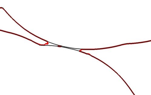
Figure 2: This is an example of a topology error fixed in step 5. The initial contour is the red line. The black line is the corrected line..

6. Equidistant points are inserted

The limit line is examined again. This time the nearest base point of neighboring limit line points are examined. If two neighboring limit line points are closest to two different baseline points, an equidistant point is inserted between these two points. (Sometimes more than one point will need to be inserted). An equidistant point is calculated accurately, and it has an accurate distance to both baseline points. Special care has to be taken to handle straight baselines.

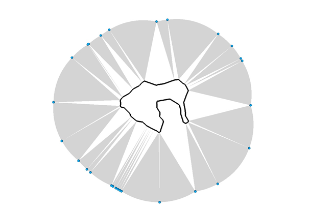
Figure 3: The blue points are equidistant points. They have the same distance to two base points.

7. The distance line is resampled.

The distance line is examined again. The distance line is now build up of several arcs from normal base points and straight line pieces from straight base lines. New points are inserted on the distance line where the arcs, and line pieces are longer than the desired limit line point spacing. These points are set accurately along the line.

8. Final adjustment to of distance line points.

In the end, step 4 is repeated. The final point position is set with the correct distance from the base point.

Details on straight base lines.

Geocap can create distance lines from straight base lines. Here is a short summary of how the normal distance line calculation was modified to handle straight base lines.

The first step in our calculation is to resample straight base lines by inserting new points on the geodesic between the end points of the straight baseline. The resample point spacing is calculated so that the error in using the resampled points instead of the real geodesic is small, compared to the distance line we want to calculate.

The resampled points are then treated as normal base points in the distance grid step (step 2 in the algorithm overview).

After an initial line has been generated, we will examine each point on the limit line, and do final adjustments to the each point coordinate. (step 4 and 8 in the algorithm). In this step we treat the distance points based on a straight baseline in a special way. We ignore the resampled straight baseline points. Instead we use an algorithm which will locate the nearest point on the straight baseline geodesic to the outer limit point we want to adjust. We then use this point on the geodesic to do the final adjustments to the distance line point.

This special treatment of distance points from straight base lines is only done if the nearest point on the straight baseline geodesic is between the end points of the straight baseline. Before the start point and after the end point of the straight baseline, the distance line is rounded off as if the endpoints of the straight baseline were normal base points.

Figure 4: Straight baselines are rounded off as a normal baseline at the end points.

Special care also has to be taken when inserting equidistant points.

Three different algorithms are used depending on the baseline type.

• Crossing point of the distance lines from two normal baseline points
• Crossing point of the distance lines from one normal baseline point and a straight base line
• Crossing point of the distance lines from two straight base lines.

A point is also inserted at the transition between the straight distance line and the arc projected from an end point of a straight base line. This is illustrated in Figure 4.