Shelf - Technical Details

Computing the gradient and the change of gradient

In this section two methods for calculating the change of gradient are introduced. The first algorithm; "Finite differences" is quite commonly known. The second one is introduced by Geocap, and therefore described in more detail. It is called the "Geocap change of average gradient" method. Both of these methods can be used in Geocap's Bathymetric profile analysis tool.

Finite differences

When approximating the derivative using finite differences, the algorithm is similar to the definition of the derivative except that because the function is not continuous, the limit value which tends towards zero is exchanged with a finite difference.

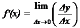
is replaced with

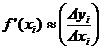
where and

This is known as the forward finite difference method. A similar method which involves and is known as the backward finite difference method. The second derivative may be calculated by using the result of one method as input to the other.

It can be proved by use of Taylor's Theorem that this approximation gives good results if the input points are regularly sampled ( )

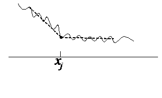
It is important to note that the second derivative at the point only involves the value at and two of its neighbouring points. The algorithm is therefore very sensitive to local variations and noise. This is why an alternative algorithm using more input points and examining the average steepness over a larger interval has been developed.

Geocap Change of Average Gradient

The change of average gradient was developed by Geocap when having been confronted with the need for a method working on a larger interval than the finite differences method. In order to compute the change of gradient at a point, the method uses the average gradient in a given interval before and after the point, and compares the two to determine the change of gradient in that point.This algorithm can use three different methods for computing the average derivative at an interval:

Method I

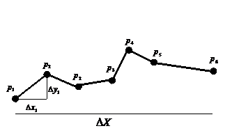
The bathymetric profile is given by the points . Let be the piecewise linear polynomial which interpolates the points

Let , and , and , and .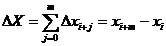

We know that because is piecewise linear , when , lets call this derivative for .

The average gradient of f between and can be computed by summation of the derivatives in the interval, weighting them by the length of the respective interval, and dividing the sum by the length of the total interval. That is: 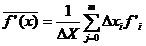by substituting with its definition, we find that: 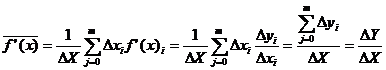where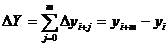

We are left with:

Method II

Let the bathymetric profile be represented by the function . is computed by studying the derivative of a linear polynomial where: and 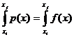where .

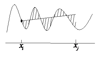
In other words, the area between and above is equal to the area between and below .

Method III

The third method uses a "Least squares" approximation of the points in the interval. This is a common method to find the best fit of a straight line to a set of points. 

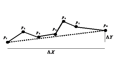
A comparison of the three methods

A less technical way of describing the algorithms will be that "Method I" is connected to the input bathymetry in both ends. "Method II" is connected to the bathymetry in one end. "Method III" will not be connected to the input line in the end points. 

All three methods will in most cases produce a similar result. However in some cases there might be differences. The three methods are less sensitive to noise in the input data in increasing order. Method 1 is more sensitive to noise than method 2 , and method 3 is the least sensitive to noise in the input data.

Computing the change of average gradient

The algorithm for computing the change of average gradient can use method one, two or three for the gradient calculation. For each point on the input line, the average gradient is computed on an interval on each side of the point, and the change of gradient computed by:

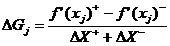
Where is the length of the interval after and is the length of the interval before . is the average gradient in and is the average gradient in

The results are similar to the second derivative of the input function, except that the algorithm identifies changes in tendencies, rather than local variations. The sensitivity of the algorithm is adjusted by changing the size of the average gradient interval.

If the average gradient calculation interval is set to the sampling rate of the input points, the change of gradient is reduced to the finite difference method.

Computing interval velocity

This section contains some technical details on how Geocap computes interval velocities in the bathymetric profile generation.

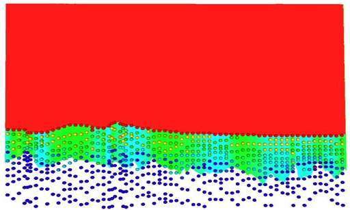
A bathymetric profile. The points are dix interval velocities, based on stacking velocity analysis

A stacking velocity analysis is done on some shot points, often with a regular interval along the seismic line. The results of an analysis at a shot point are several velocity picks, where each velocity pick consists of a z-value in TWT and the stacking velocity at this z-value for the shot point.

In deep water the stacking velocity will coincide with the RMS velocity. Based on RMS velocities the interval velocities on the same picks may be computed using Dix's formula. The result after running Dix's formula on an RMS velocity dataset in Geocap, or a Stacking velocity dataset as a substitute, is a dataset where each velocity pick now contains the Dix interval velocity for the interval between the pick and the pick above.

Geocap can create a velocity profile based on the interpreted horizons and the corresponding Dix interval velocity dataset. This is done using the "Generate Velocity Profile" command.

Based on Dix interval velocities the interval velocity in the interval between the interpreted horizons may be computed at the shot points with a velocity analysis. This is explained in the in following section. After this, the velocities for the rest of the points on the interpreted horizons not containing a velocity analysis are computed. This is done by interpolation and extrapolation. For points on the horizon between two velocity analyses, velocities are interpolated using a linear interpolation between these analyses. Some points on the interpreted horizons are only related to one velocity analysis. This is the case at the beginning and the ends of the seismic line. In these cases, the velocities from the nearest velocity analysis are used directly.

Interval velocity generation

At a shot point with a velocity analysis, interval velocities in the interval between each of the interpreted horizons are computed. The simple case is described first. Next a couple of points which may complicate the simple case are mentioned.

The basic idea is illustrated in the figure below:

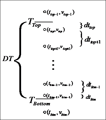
is the TWT at the first interpreted horizon.

is the TWT at the second interpreted horizon.

The Dix interval velocity picks are represented by the small circles, and TWT velocity pairs.

is the first velocity pick after

is the first velocity pick after

when

Note that

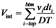
The interval velocity in the interval between and is

and is given by the following formula:

Distance Calculations

Geocap uses distance calculations in a number of different algorithms. Some used to calculate distances between points, other used to generate a distance line at a certain distance from a point or line.

In these algorithms you can choose which distance calculation algorithm you which to use. Here is a description of the different algorithms:

Flat Earth

The flat earth calculation will calculate a distance based on the coordinates of the current projected coordinate system. The distance calculation will be based on Pythagoras theorem on the coordinates. The accuracy of this calculation compared with the shortest distance on the earth ellipsoid will depend on the projection.

Ellipsoid Approximation

This algorithm based on a formula in the book "Astronomical Algorithms" by Jean Meeus (page 85). He refers to H. Andoyer and "Annuaire du Bureau des Longitudes pour 1950 (Paris), page 145" as the source of this formula.

The relative error of the result is of the order of the square of the Earth's Flattening.

An example in the book computes the distance from Observatoire de Paris (France) and the U.S. Naval Observatory at Washington D.C. (6181.63 kilometer). According to this book, the distance calculation has a possible error in the order of 50 meter. (0.0008% of the total distance in this example)

Vincenty's formulae

This is the formula with the best accuracy available in Geocap. It is accurate to within 0.5 mm (0.020″) on the Earth ellipsoid

See

http://en.wikipedia.org/wiki/Vincenty's_formulae

for more information.

The calculation of the 2500 meter isobath

The 2500 meter isobath can be calculated on two different types of data: lines (polydata) or grids (structured points / rasters).

2500 meter isobath from lines:

For lines Geocap will make a new point dataset with points inserted where the line crosses the 2500 meter depth. A line is built up of points, and it will probably not have a point at exactly 2500 meter depth. Geocap uses a linear interpolation between the two nearest points on the line where one is shallower than 2500 meter and the other is deeper than 2500 meter.

The result is a new dataset with points where the line crosses 2500 meters. 

2500 meter isobath from grids:

For grids, Geocap will perform a contouring algorithm of 2500 meter on the dataset. This is done on the the full resolution of the grid.

Geocap uses an algorithm very similar to the well known "Marching Squares". However when a line piece is to be inserted, Geocap will split the square into two triangles. The inserted line piece will be put on a linear interpolation between the corners of the triangle. A 2x2 set of grid nodes can be split into triangles in two ways; by joining the top left node to the bottom right node, or by joining the top right node with the bottom left node. Geocap will consider both ways, and choose the one which would be used if the grid was to be triangulated. The triangulation algorithm will compare neighbouring nodes to the 2x2 block and choose direction on the triangle based on the gradients in the corner points.

The resulting line will have one additional point for each 2x2 block of grid nodes compared with a regular "Marching Squares" algorithm.