Digitizing the Outer Limit Line

Introduction

This article will present in detail the keyboard functionality that will assist the user when digitizing the new outer limit line to get a preliminary result. The case study is taken from the Atlantis demo project so that everybody can train themselves by following the exact same procedure.

Outer limit lines are calculated according to the geodetic settings of the dataset found under Properties. One should as a quality control do a check of the lines to secure that they can be used as outer limits. The spacing of points should be within reasonable size to secure accuracy. 1000 or 2000 meter is often found appropriate.

On this page:

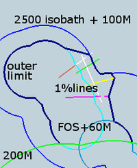
In the Atlantis project, the Outer Limit Generation menu is activated by right clicking on the folder 4. Outer limit, and choosing the Generate Outer Limit command. The menu shows the data sets in the Constraints, Formulae, and Outer Limit folders (note that all formula and constraint lines to take part in the combination procedure should be copied from the appropriate folders in the project and pasted into the corresponding folders in 4. Outer limit before proceeding). The outer limit line will be generated from a combination of these formula and constraint line pieces. Place a check mark next to the data sets in the Generate Outer Limit menu you would like to display and click on the pencil icon to show the actual lines in the display window.

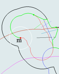
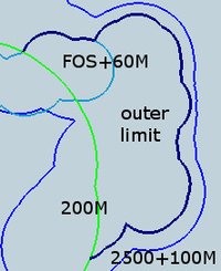
The lines in the picture are the various limit lines that are used for combining the new outer limit line. The different limit lines are indicated by text. The constraint lines consist of the baseline + 350 mile line and the 2500 meter isobath + 100 mile line. The formulae lines consist of the baseline + 200 mile line and all the FOS + 60 mile lines plus the 1% sediment thickness lines.

Starting digitizing

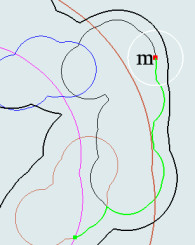
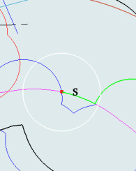
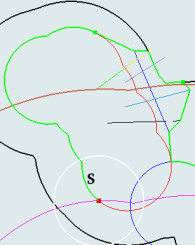
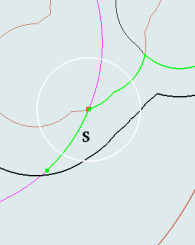
The start point for digitizing is indicated with a marker and the text Start in the image. We begin at the crossing point between the 200 mile line and the FOS + 60 mile line. To start just activate the Digitize entry. The screen will then be set in 2D mode so that a single click with the left mouse button is enough for the primary digitizing which will attach the first point in the digitizing line to the nearest point on any curve from the cursor.

The circle with radius 60 mile

The digitizing procedure will display a circle at the last position. The radius of the circle is the maximum distance that points are allowed to be separated and will serve as a guidance when digitizing and connecting to other points.

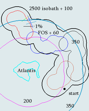
Various lines used for combining the outer limit line

The shortcut keys are essential for fast and precise digitizing. They will be demonstrated and explained throughout the exercise.

The procedure when applying a shortcut key is very important: The graphical screen must have focus. That is achieved by clicking at the toolbar of the screen or zooming slightly in or out with the right mouse button. Then place the cursor (as an example) exactly at the crossing point in the screen and press c on the keyboard. The same procedure goes for all the keyboard strokes. Over again, the screen must have focus for the shortcut keys to work.

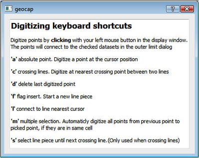
Keyboard shortcut keys in digitizing

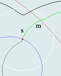
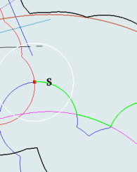
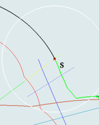
1. In this study we have to apply the keyboard c to get the start point, the crossing point between the 200 mile and the FOS + 60 mile lines. We zoom in as closely as possible to position the cursor exactly at the crossing lines and hit c to generate the crossing point.

2. The s key will select the line piece from the last position to the first crossing line. In this case the green line shows that a line piece is selected until a new FOS + 60 mile line is met. Look at the overall display to get the picture right.

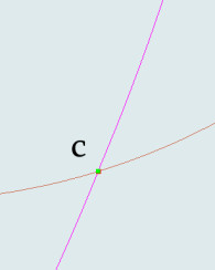
1. Using c to get the crossing point

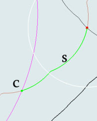
2. Starting with c, then using s

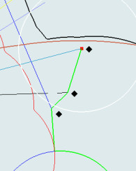
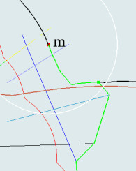
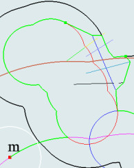
3. The m key will select points in the line from the last position until the point nearest the cursor where the m key was activated. Notice that the FOS + 60 mile line is a closed line so that the selected line piece could have been to the left or to the right. The selection is always using the shortest distance. Therefore the m key was applied far out, but still below half way of the closed line.

4. The digitizing continues with m for multi selection to a specific position. The position is intentionally selected to be after the 350 mile line so that it is possible to use s in the next operation.

3. Using m for multi selection

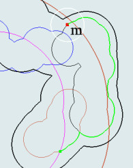
4. Using m for next multi selection

5. As indicated, the next shortcut key is s for selecting until first crossing line which is a FOS + 60 mile line.

6. Next we are doing an optional ending at the 200 mile line. This part of the digitizing is very appropriate for applying s. We utilize that there are crossing lines and the outer limit line will go exactly to the crossing point and continue in a new line. In this case the s key connected the outer limit line to the 200 mile line.

5. Using s for selecting line piece

6. Using s for selecting next line piece

7. It may be a practical question if the line should have stopped at the 200 mile line, thus breaking up the outer limit line, because the 200 mile line is not part of the new claim. In our case study we go on with the digitizing and incorporate the little part of the 200 mile line. The s key is used over again to incorporate a little piece of a FOS + 60 mile line.

8. The s key is used over again to incorporate a little piece of a FOS + 60 mile line.

7. Using s for selecting next line piece

8. Using s for selecting line piece

9. Next we want to attach to 1% sediment thickness lines. The three dots indicate that one can just click with the left mouse button to attach to the outermost point in the 1% sediment thickness lines.

10. Now the digitizing has come to the end point of the 1% sediment thickness line and one wants to proceed to another end point of the same kind. But in that case the line will be outside the 2500 meter isobath + 100 mile line. It is therefore appropriate to use the l key to connect to the isobath line in the very straight line direction to the end point of the 1% sediment thickness line. The reason for using l is that this shortcut key will connect to a line at the exact cursor position, and not use the nearest point that otherwise would occur if one just clicked on the line.

Another question is how do we find the exact direction during digitizing. In this case we just zoomed in and used a ruler on the screen. That is the quick way to do it. A more correct way is to prepare those cases with lines on beforehand and display those lines as a guidance.

9. Left mouse click for selecting points

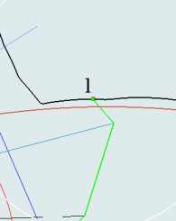
10. Using l for connecting to line

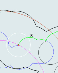
11. The digitizing continues with m for selecting points on the 2500 isobath + 100 mile line. We place the m just before the last crossing of the isobath and the 1% sediment thickness line because after that we have to go away from the isobath line.

12. We use s to select the line piece until the 2500 isobath + 100 mile line crosses the outermost of the 1% sediment thickness line.

11. Using m for multi selection

12. Using m for multi selection

13. Investigating the line situation we see that we have to leave the isobath line and pick up the next endpoint of the 1% sediment thickness line. That is done with an ordinary left mouse button click.

14. The digitizing has come to the last point in the 1% sediment thickness line and shall continue. The nearest line in question is a FOS + 60 mile line. In this case the white circle is of great help because it tells exactly how far out the connection can be. We use the l key exactly where the circle crosses the FOS + 60 mile line.

13. Left mouse click for selecting point

14. Using l for connecting to line

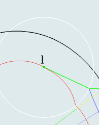
15. We continue with the m key for selecting points on the FOS + 60 mile line. The selection is beyond the first crossing line to establish the starting point for the next selection.

16. The next picture shows that we can follow the FOS + 60 mile line to the crossing of the 200 mile line. Thus we use the s key.

15. Using m for multi selection

16. Using s for selection onto 200 mile line

17. We could have stopped here because the new outer limit line seems to be complete. But as an exercise and also as an option we continue a little on the 200 mile line. That is done with the m key.

18. The picture shows the result so far with all limit lines displayed and the outer limit line in green. At this stage we see that the start of the digitizing doesn't harmonize with the end.

17. Using m for multi selection onto 200 mile line

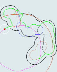
18. All lines displayed with dig line in green

19. As a further exercise we want to attach a little piece of the 200 mile line at the beginning of the digitized line. We then use the f key to introduce a flag in the digitizing so that the line is broken up. After the f key we just left click on the 200 mile line at a suitable point to connect the digitizing to this line at the nearest point.

20. We use the s key to connect the digitized line to the first crossing point. In fact the same crossing point where we started.

At this point the digitizing is finished and we click End digitizing in the menu and save the data as Digitized Outer Limit. The line schema is Limit Line, but we temporarily set it to PolyData in order to utilize the Additional Display options, especially Cells in different colors.

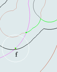
19. Using f for inserting a flag

20. Using s for selecting line piece

21. The picture shows the line situation. We have got two cells in the line. This is not as it should be. A line that is supposed to be continous shall contain only one cell. We therefore want to sort the two cells into one.

22. Sorting of line pieces is done by the command object Utilities > Sort line pieces into cells. The schema must be PolyData and the proper command objects in Operation Modes must have been activated for this command object to be visible. The sorting works so that all line pieces that are in different cells but have common connection points with adjacent cells are combined into a common cell. In this case the two line pieces are combined into one.

We have digitized the outer limit line to be just one line piece. This is an option. If one choose to have several line pieces; for instance to stop at the 200 mile line, those line pieces must be digitized separately and saved as individual lines. The treatment afterwards to maximize the outer limit line must also be done separately on each individual line.

21. Digitized line containing two cells

22. Digitized line is corrected into one cell

It is important to understand two prerequisites of this case study:

1. The text describes convenient digitizing elements and how to use them properly. The line can be done with other choices especially in the 1% sediment thickness part. See below for an alternative digitizing.
2. The digitizing is performed to get a preliminary result. The final result is done by carefully closing bays with lines up to 60 mile of length. This can be done interactively with the command Maximize outer limit. This command object requires a Geocap version of 4.3.7 or higher. There is a complete explanation of that procedure in the text Maximizing the Outer Limit Line.

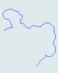
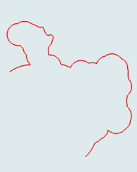
As indicated in the exercise the digitizing could have been performed consequently to start at the 200 mile line and ending at the 200 mile line without including that line. The outer limit line would then have to be digitized in two parts for the Atlantis demo project. This was also done in another quick exercise and the result is displayed in the left and right pictures.

The digitized line in the area of the 1% sediment thickness was optimized a little bit better which illustrates the complexity and planning of a proper outer limit line generation.

West digitized outer limit line

East digitized outer limit line