Gridding seismic interpretation with faults
- Former user (Deleted)
- Erlend Kvinnesland
Abstract
Case: A set of seismic lines for a certain horizon has been interpreted in Kingdom Suite. Also fault line traces are interpreted. The lines are read into a Geocap project.
Purpose: The data will be analyzed and edited to make them suitable for gridding in Geocap. The documentation will describe errors and inconsistencies in the data and how to clean and edit the lines in order to get a good gridding result.
On this page:
Triassic demo project
A demo project called Triassic demo was created with the initial seismic lines and faults. The picture below shows the project and the initial interpreted lines and faults from Kingdom.
The text follows closely what happened during the work.
Disclaimer
Due to a substantial amount of errors in the seismic lines and fault traces, a large part of this case study deals with correcting the errors. The way it is corrected is in principle simple, but requires an suitable knowledge of Geocap functionality which consequently is presented during the text.
Having corrected the errors on the input datasets, the gridding is straightforward and explained in detail by menu images. Geocap has a unique fault gridding algorithm for incorporating fault traces into the result grid surface.
If needed, there is also an option that Geocap personnel can assist in practical work if necessary when a similar project has to be performed.
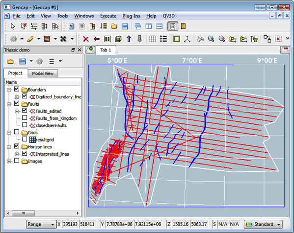
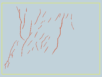
Seismic lines and faults displayed in Geocap, but interpreted in Kingdom
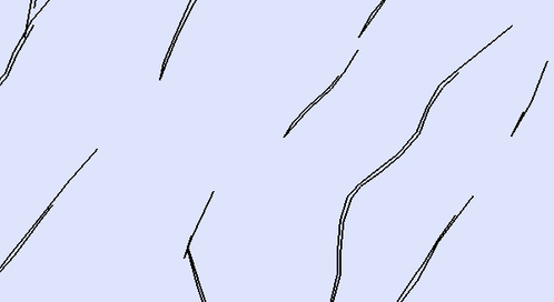
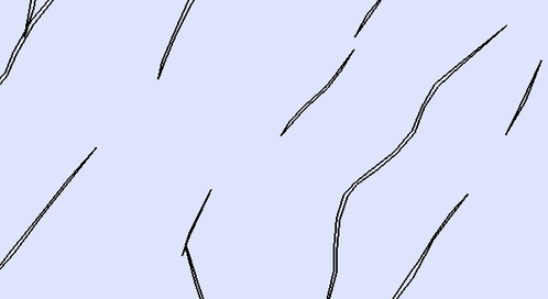
Error in seismic lines
Analyzing the seismic lines closer it reveals spikes. In the table view one sees the z-values for the spike points are -999. An error has been introduced somewhere in the process of saving or importing the data. No matter what the reason is the spikes must be removed. The easiest way is to mak the dataset active and eliminate the spikes with a shell command:
- Interpreted_lines->Make Active (will transfer the lines into active data)
- In the shell: eli lt 0 ; # eliminate z values lower than 0.
- Interpreted_lines->Assign Data From ...->active (will transfer the lines back into the project)
- The input also showed three very long lines with just start and end points. These line were deleted using:
- mak cel dis 30000 ; # make a new cell if distance between points are greater than 30000.
- The lines were then assigned back to the project.
The interpreted lines are now cleaned and updated.
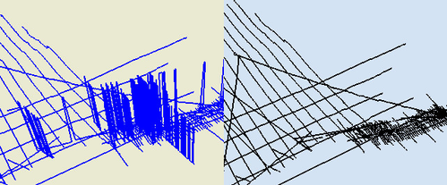
Seismic lines before and after eliminating spikes
Error in faults
Fault traces that are gridded in Geocap can be:
- Single lines traces. Z value of no importance.
- Closed lines traces without using z values (or just 0 in z values).
- Closed line traces with z values.
The fault traces in this case are closed line traces without z values. However, they display with fault throw boxes and are not suitable to be used in the fault gridding. They are also not properly closed. Ergo, the following work must be done:
Error correcting tasks
The fault throw boxes have to be deleted and the lines traces must be closed.
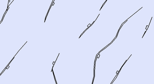
Fault traces with fault throw boxes
Deleting fault throw boxes
There are two ways of deleting the boxes:
1. The first way to delete the fault throw boxes is simply to delete them interactively:
Faults_from_Kingdom->Edit points and lines - Delete - Repetitively - Delete all points in a cell - Start delete. Stop delete.
This method is applicable when the fault throw boxes are separate cells (as in this case). If the fault throw boxes are part of the fault traces (which often is the case) one has to delete the individual points.
2. The other way to delete the fault throw boxes is to use a shell command for quick removal of points. The first observation is that the fault throw boxes are separate cells and each cell has four points. If no fault traces has four or less points one can delete all cells containing points lower than five.
The command for deleting all cells with less than five points is:
del cel lt 5 nr ; # delete cells with less than 5 numbers. 52 number of cells were deleted.
However, two fault traces was also deleted as the picture to the right shows.
The new trimmed fault traces were added back into the project. Then the two fault traces that also were deleted are selected from the original dataset by the command object Edit points and lines-Select-Select Cell . For each selection the command object Append polydata from workspace was used as shown below. The edited fault traces are saved in the project as Faults_edited data.

Menu for appending selected data to the fault set
Close the fault line traces
Looking at the fault dataset after removing the fault throw boxes one sees that the traces are not properly closed. Make the fault dataset active and do the command in the shell:
mak cpl ; # make closed polygon .
All but two fault traces were properly closed. For these two exceptions they were closed with Faults_edited->Edit points and lines-Digitize-Start. Use keyboard n for connecting to the nearest point and close the remaining gaps. Use keyboard f between the cells. Finally the fault trace picture looks correct as shown in the picture to the right.
The fault traces are now ready to be used in fault gridding. To check that they are correctly edited one usually perform the bmo test; i.e. grid the fault traces within the grid window with the bmo command. That test is also part of the gridding panel in the fault menu page. Grid cells should only be present inside the fault traces for a proper gridding of seismic lines and fault traces.
Result of deleting cells with less than five points
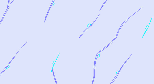
When the fault throw boxes are deleted the zoomed-in fault display should look as below.
Fault throw boxes removed
Fault traces finally edited
Gridding of seismic lines and fault traces
The gridding menu is activated on the interpretation lines. The front menu panel is shown in the image to the right.
The Grid Window menu must have correct values by the following procedure:
Steps in setting up the grid window
- Scaling the window to the digitized boundary. This is done by
Digitized_boundary_line->Zoom to Data - The button Use Active Window was applied to transfer the generated window to the menu. The grid model will take place inside the grid window.
- The x and y increments of the grid was set to 200.
- The Calculate button was applied to get the number of elements in rows and columns.
- The button Adjust to Increment was applied to set the grid window to be aligned with the increments. It is recommended to have the grid window adjusted to the increments.
- Draw Window Frame was applied to check that everything looks ok.
- The type of data was set to 2D seismic lines.
When all parameters in the grid window are in place it is then ready for the fault menu page.
The Fault Input menu page shows in the image below:
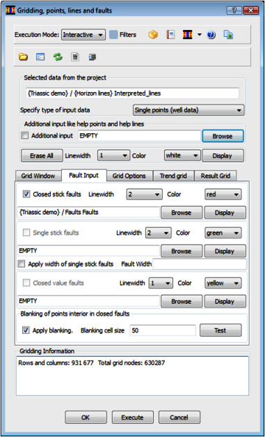
Fault menu page

Grid window menu page
The closed stick faults that was edited and cleaned up are browsed into the fault page. The option Apply blanking is checked in and a blanking cell size of 50 is selected. To check the blanking of the closed polygon fault traces the Test button is applied to show the graphical result. This test is sometimes called the bmo test after the bmo command (border modeling) which performs the grid model inside the faults. The result looks like the image below.
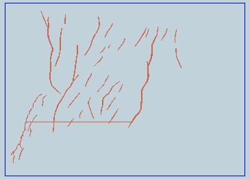
Result of the test of closed fault polygons
The bmo test shows that there is a long horizontal line that indicates an error somewhere. Such lines can occasionally occur in x and y direction and are due to incorrect lines of some kind. It has to be investigated by checking especially the start and end points of the erroneous line. A zoomed in display of the leftmost position reveals the cause:
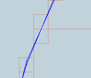
Zoomed-in detail of fault lines crossing each other
The fault traces are crossing each other and incidentally a grid line is going exactly at the crossing point. It is a small matter to move one point in the fault trace to get it correct. Apply Edit points and lines and use the Move option. The detail now looks like:
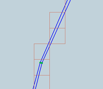
Detail of corrected fault lines and fault grid
Performing the bmo test over again the picture of the fault traces with grid cells look like:
The fault traces are now completely correct to be used in the fault model gridding. The fault traces are modeled with the option of including the boundary; that is why even thin parts of the closed fault traces have grid cells around.
Correct fault test showing fault grid cells
The next step is to go to the Grid Option page which looks like the image to the right.
The digitized boundary line is browsed in to be used as an outline for the grid. We also apply two step gridding which usually is advantageous when gridding seismic lines. The first step grids with a coarser grid, then removes points laying close to the input, and append what's left with the input. Then the second step is performed. Areas far away from the input lines will thus be stabilized.
The increment of the first step was set to 1500 which is in the recommended range of 3 - 10 times the size of the final grid increments which in this case is 200.
The interpolator for the first step was selected to be moving average and the second step applied parabolic interpolation.
The result is a grid of good quality with sharp defined faults.
The grid was displayed with the command object General Display using a combination of color bands and line contouring to get the highlighted contour lines. The white fault traces are added (or saved) to the project from workspace where they are called closedGenFaults.
The Result Grid page is not shown in this text as it is easy to understand. One has the option to put the result data directly into the project or have it only saved in workspace and add it to the project afterwards.
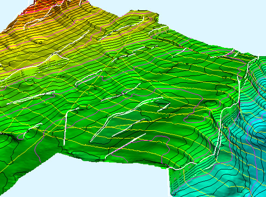
Surface result of gridding seismic lines and faults
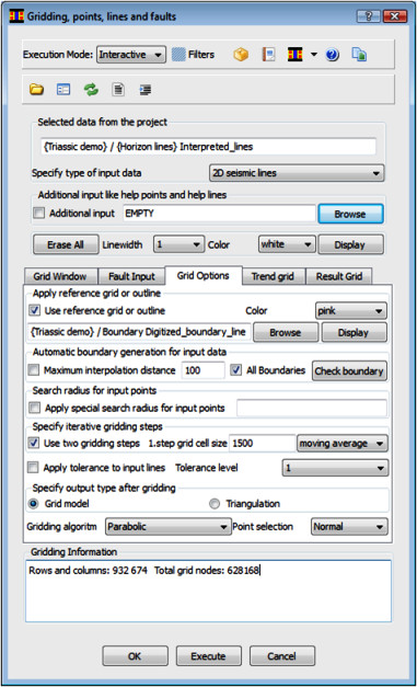
Grid options menu page
Conclusion
The text in this documentation shows the principles of data cleaning using command objects and some smart shell commands to do effective work. The use of shell commands is an option and is meant for direct action and shortcut in some cases. There is normally an equivalent in a command object using a menu. In this text a few shell commands are presented to show their use.
Gridding of interpretation lines and faults requires input data of high quality. The fault traces should be properly closed with no fault throw boxes. It is a necessity to master the editing of input data to get it all correct before gridding.