Gridding and surface modeling tutorial
- Erlend Kvinnesland
- Olav Egeland (Unlicensed)
- Former user (Deleted)
Introduction
Gridding is the process of transforming data points in different forms like scattered points or line data into a regular grid of node values. Read about gridding in the main documentation.
The gridding process is suited the needs and requirement in oil and gas exploration where subsurface horizons are modeled and a reservoir model is constructed. Gridding in the Seafloor module of hydrographic survey data is another story and should be handled accordingly.
Tutorial steps in gridding
In this tutorial we will investigate the gridding process and algorithms by some educational steps.
Tutorial procedure
- To make it simple and still somewhat realistic we will start with random points and grid these into a surface.
- Then introduce some fault lines to see the effect.
- Next step is to generate some sample lines from the first surface to simulate 2d seismic lines.
- The 2d seismic lines are input to gridding to demonstrate gridding of 2d lines with faults..
- All data involved will be saved in a project and the workflow and menus involved are the standard ones used in Geocap and can be utilized in similar cases in real life.
The user is encouraged to follow the tutorial steps and repeat all the tasks that are performed. It will then become a valuable training session going though some of the kernal elements of the software.
On this page:
Preparation
Creating a new project
Begin this tutorial by establishing a new project called Gridding demo. Start with one Generic folder.
Establish a grid window
The grid window is important when gridding. In this tutorial we select a grid window that has realistic coordinates i x, y and z:
xmin=450000 xmax=460000 ymin=6450000 ymax=6460000 zmin=1000 zmax=4000
This grid window is for convenience established using the command: win demo. Do that command in the command shell.
Go to the Project Settings on the project tool bar and under Data and click Use current. Likewise, under Graphics select white as background color and check in the two boxes Erase graphics when loading project and Apply settings when loading project.
We use these options in our tutorial as they are convenient when loading the project.
Gridding of a few scattered points
Create some random free points
At this step the task is to generate a few random points with the grid window. These points would then represent surface data or well data. In the demo case 11 random points were generated using the shell command: mak ran 11. Create a folder called XYZ data in the project and apply New -> Workspace Data -> Active. Rename the dataset to well data.
Check that the random points have a reasonable distribution across the graphical window. If not repeat the generation.
Digitize a surface boundary
In order to be more realistic we want to generate a boundary for the reservoir surface. This is done using the digitizer under Tools -> Quick Digitizing.
Digitize a closed boundary going fairly close to the edges and including all points to get a good representation. In the default case when ending the digitizing the digitized line is saved in workspace as digitized_line.
Establish a new folder called Boundary and put the digitized line into that folder using New -> Workspace Data -> digitized_line. Rename this dataset to border line.
For convenience establish a folder called Images to capture screenshots along the development of the project and the tutorial. For later use a folder for Grids and a folder for Fault lines are created.
It all looks like this:
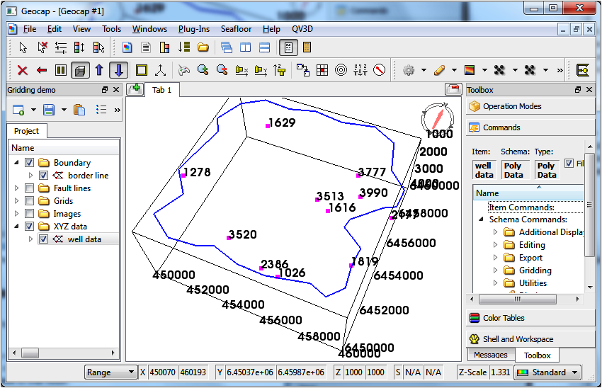
Dispay of project and graphics when staring the tutorial
Generate a grid surface from scattered points
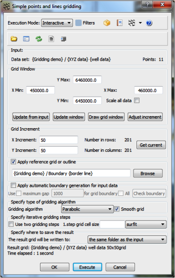
This task is simple. We prefer to apply the command Simple points and lines gridding found under Gridding.
Fill in the menu as shown to the right and perform gridding. The result grid will be placed in the same folder as the input. In this case a new folder was established called Grids and the generated grid was cut and pasted to that folder.
The result grid is mapped below with Map Data. The input points are displayed for reference and one sees clearly how god the interpolator honors input data. The color legend was displayed using a little script that is explained below.
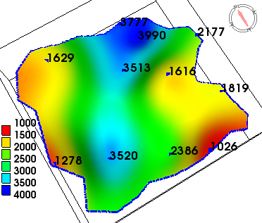
Gridded surface from a few scattered points
To get the graphics suitable for presentation as with this tutorial the ambient light was set up. Default is 0.2 and the shell command amb 0.3 was applied. The reason is that presentation graphics may benefit from more ambient light although it is a matter of preference. But try it out yourself and make an evaluation.
Generate a color legend script
The color legend was displayed using the shell command cco s 1000 500 4000 rev col bla. For convenience this color legend command was placed in an item script for the grid surface and called Color legend 500 inc.
Establishing small scripts are effective in real production cases and is part of this tutorial. The way it is done is as follows:
Establish a color legend command script
- Place the cursor on the grid surface so this is highlighted.
- Go to Item Commands under the Commands section and activate ->New Command.
- Find Script and click OK.
- Rename Script to Color legend 500 inc and click OK.
- Edit the script and write in the color legend command: cco s 1000 500 4000 rev col bla.
- This color legend is now suited for the particular grid surface.
Show results with different algorithms
The gridding was repeated with two other algorithms: Moving average and Surfit. Read more about gridding algorithms in the user guide.
The three surfaces were collected in the Grids folder and renamed to: gridmav gridpara gridsurfit. A command script located on the Grids folder and called Grids in viewport was created to display them in a connected viewport presentation. The script is simple and explained below.
The script is executed on the Grids folder. That means it will execute the contents within the Prestep just once. The contents within Main is executed on every dataset in the folder. The contents in Poststep is executed finally just once.
Here is the contents in Prestep. An initial variable is allocated and the viewport arrangement is achieved. This is done before any execution on the datasets.
# This is the contents in Prestep
variable init 0           ;# initialize an init variable

vie def                   ;# reset viewports to default
vie 3 1 1                 ;# allocate 3 x 1 viewports
Here is the contents in Main. It selects the viewport number and performs the mapping and other graphical stuff. Beware that the well data is copied and pasted to workspace where it get the name welldata having no blanks in the name. Then it is easy to apply the well points in the script.
# This is the contents in Main
incr init                ;# increment init variable
spe amb 0.3              ;# specify overall ambient light 0.3
vie $init con            ;# go to viewport number in variable and connect to previous
spe bgc ran lig          ;# specify random background light with a light value
col bro                  ;# select brown color
dra win                  ;# draw graphical window
map rng 1000 4000        ;# map using range values
col blu                  ;# select blue color
bol 2                    ;# draw border of the grid with linewidth 2
mlo welldata             ;# move welldata to active which has been placed in workspace
col bla                  ;# select black color
poi                      ;# display the points
if {$init == 1} {                         ;# chech on init variable
    tx2 lle col bla txt "Moving average"  ;# the first is moving average
    cco s 1000 500 4000 rev col bla       ;# display color legend
} elseif {$init == 2} {                   ;# the second is parabolic
    tx2 lle col bla txt "Parabolic"       ;# display text in 2d mode
} else {                                  ;# last is surfit
    tx2 lle col bla txt "Surfit"          ;# display text in 2d mode
    mak com                               ;# make the compass and display
}
No statements are necessary in Poststep.
The user may copy these statements and put them correctly into the script and reproduce the display.
The viewport display is taken out as a screenshot and saved. The result shows that the algorithms solve the interpolation task slightly different. Such a difference is more obvious for few points where the degree of freedom is greater.
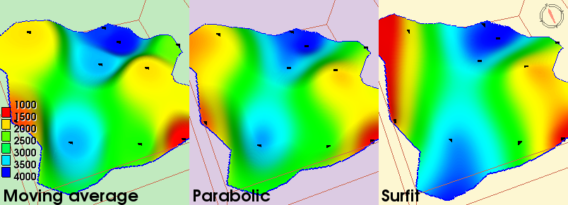
Viewport presentation of gridding with different algorithms
To go back to one viewport use the viewport icon on the toolbar or type vie def in the shell. To set white background go the the project toolbar and activate the project settings or type spe bgc whi in the shell.
Introduce some stick fault lines
The next task is to show gridding in combination with fault lines. Geocap can handle this type of fault lines:
Three types of fault lines
- Single stick faults. Just plain lines with no z values.
- Closed stick faults. Closed lines representing upper and lower fault trace. No z values are given.
- Closed faults with z values. Closed lines representing upper and lower fault trace with correct z values.
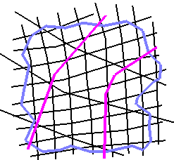
In this case two single stick faults were digitized as shown in the picture. They were placed in a new folder called Faults.
The stick faults were digitized with an eye on the well data values so that a natural fault pattern would be achieved. Do the same with your data.
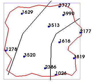
Two stick faults digitized among the well data
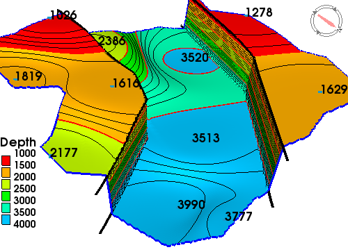
Generate grid surface with faults
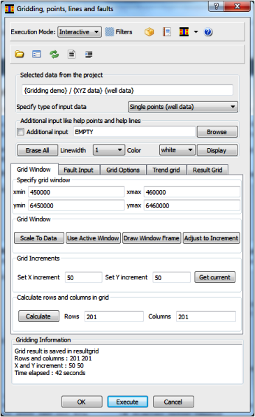
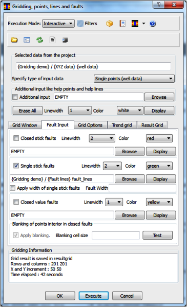
To generate a grid surface using faults as extra input one has to apply the menu Gridding, points, lines and faults found under Gridding.
The menu settings should be fairly straight forward. The two menu displays shows the Grid Window page and the Fault Input page settings. Otherwise it is default settings with the exception that smoothing is turned off on the Result page. The result grid will by default be saved in workspace resultgrid so we pick it up from there after the gridding.
Gridding is performed using the single stick fault lines as blocking lines so that the evaluation of any grid node is only affected by input points that are within non blocking connection with the node.
After gridding transfer the resultgrid in workspace over to the Grids folder and rename it to resultgrid_faults.
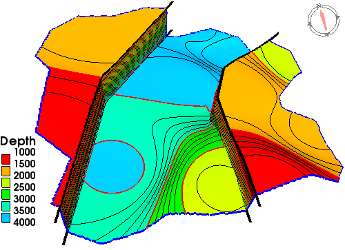
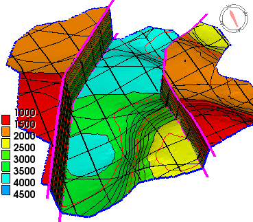
The result grid with faults shows a good sharp edge where the stick fault lines were placed. The algorithm generates an upper and lower fault trace that is saved in workspace closeGenFaults. That dataset is transferred to the Fault lines folder and displayed in black in the display.
The mapping was done with the command Additional Display -> General display applying a combination of Color bands and Line contours. Color bands is applied with increment 500 (and no checkbox for Draw contour lines) while Line contours applies an increment of 100.
The right display shows also the input points and tells that they are honoring the derived surface.
Exercise - Make a grid surface with faults and apply Two step gridding
- Make more random points (for instance more than 20).
- Introduce several single stick fault lines; some shorter and some longer.
- Use the described procedure so far to generate the surface with faults.
- Apply Two step gridding option for better grid results,
A new exercise was performed which is displayed in the viewport arrangement below. The result was not good enough right away so Two step gridding had to be applied.
Using two step gridding option if problems with surface quality
- Working with random points and introducing random fault lines, problems can occur in the gridding.
- This is illustrated in the next display where 23 random surface points were generated and some random stick fault lines were introduced.
- Although random generated data are weird there are similarities to real cases where data can be very odd arranged.
- A useful and necessary option is to apply the Two step gridding option. The improved result is shown to right.
- The grid increment for the first gridding step should be from 5 to 30 times the final grid increment.
- In this case the final grid increment is 50 and the first gridding step increment is 1000.
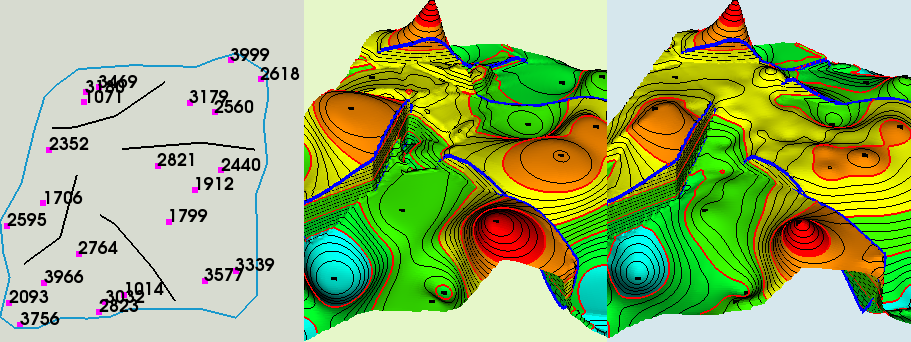
Three stages of grid exercise: 1: Input data. 2. Grid result. 3. Improved grid result using Two step gridding
Gridding of line data
This tutorial is based on creating input data along with the tutorial steps. This goes also for gridding of line data.
Tutorial procedure for gridding line data
- We will try to reproduce the first generated faulted surface using line data as input.
- The line data is supposed to represent seismic 2D survey lines.
- The following procedure should be followed:
- Digitize a representable set of lines that are supposed to be seismic 2D lines.
- Convert the digitized lines into a dense set of points along the lines.
- Sample the seismic 2D lines into the faulted surface.
- Grid the seismic 2D lines into a surface to get the faulted surface back as good as possible.
Digitize some arbitrary lines
Digitizing is as usual done with Tools -> Quick Digitizing. Here is the line set that was digitized. It is saved in a project folder called Line Data.
The digitized lines represents seismic 2D lines going basically in x and y directions. A few lines are also crossing from upper left to lower right which may be the case with 2D surveys occasionally.
Feel free to digitize the lines after your own choice. The task is to study line gridding and to see what line data input is necessary to get a good surface representation.
Digitized seismic 2D lines
Sample values to the lines from previous grid surface
The digitized seismic 2D lines is so far not quite suitable to be used. It requires more points; i.e. seismic 2D lines have a shot point spacing that we will introduced. A fairly adequate spacing is 100 meter. This is achieved quite simple using the following procedure:
Convert the digitized sample lines into a dense set of points along the lines
- Do Make Active on the digitized lines.
- Type in the shell command: mak lin dis 100 , which means Convert the points in the lines to new line points of 100 meter distance.
- Add the new dense line set back into the project. Call it f.inst. seismic2d.
The faulted grid surface generated as the first grid from surface data and two stick faults will be used as a master surface to be reproduced. Assume this grid is called resultgrid_faults. Do Copy and paste it into workspace.
To create a realistic sample set representing 2d lines do as follows:
Sample surface data into seismic lines
- The line set seismic2d with dense points is active. (Do Make Active).
- resultgrid_faults is located in workspace as explained above.
- Do the shell command: zap resultgrid_faults to sample values from the surface grid into the seismic line data.
- Save the seismic 2d lines into the project and give it the name (f.inst.) seismic2dvalues.
The illustration to the right shows the sampled results.
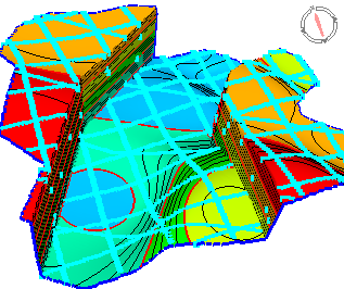
Artificial seismic 2D lines with surface values
Gridding line data with faults
Following the tutorial steps so far the line data is ready for gridding. We use as before the menu Gridding, points, lines and faults found under Gridding. It is basically the same settings as before with two extra specifications. A summary is given below.
Summary of menu settings for gridding line data
- All settings are the same concerning:
- Grid window
- Grid increments
- Single stick fault lines
- Border outline
- New settings are: Use two gridding steps. If 1. step grid cell size is left blank Geocap estimates 4 times result grid increment = 200
- Optional setting: Specify type of input data: 2D seismic lines. (If this one is omitted Geocap will find out).
The grid result (unless specified to be saved in the project) is saved in workspace resultgrid and the generated fault traces is saved as closedGenFaults. Transfer it to a proper folder in the project.
The result display is shown to the right. It shows the surface that has been generated from artificial seismic 2D lines.
Result grid from line data gridding
Regridding with different parameters
A critical parameter in line data gridding is the grid cell size value in Use two gridding steps. If it were blank the algorithm used 200 (= 4 * 50, where 50 is the result grid increment). Some other values were tried and it turned out that 200 gave the best result.
Two steps gridding works by letting the first step generate some surface points that are appended with the input lines to represent input data in the final gridding process. That dataset is present in workspace as input_data and can be inspected and displayed.
Below is a viewport representation of two result grids with different 1. step grid cell size and the original surface. A quick view valuates the first grid as the best.
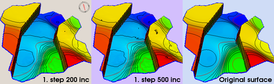
Result grid for two different cases of 1. step grid cell size and original surface
Exercise - Gridding of line data
- Make fewer seismic lines or make the spacing between the lines more unequal.
- Study the effect of gridding for different data sets.
- Try to find the most favorable value of the 1. step grid cell size.
- If necessary introduce extra lines or pseudo points to make the gridding perform satisfactory.
All the issues in the exercise are cases that can occur in realistic situations. Gridding is dependent of input data and the parameters used in the algorithm. Good knowledge about gridding will benefit a good grid result.