6. Gridding

Basic concepts

Grid window

The grid window is simply a rectangular window surrounding the grid. The grid window can be larger than the data area, but never smaller if one wants to grid all data. For grids to be compatible (e.g. to be used in grid to grid operations), it is important that they have the same grid window.

The grid window is a term that is used in two ways:

1. Before a grid is established, it is the window frame that tells where the grid will be defined.
2. After the the grid is established, it is the min and max extent of the grid in all coordinate directions.

The window frame is drawn by the frame icon . This window frame is sometimes referred to as the graphical window because it is the window one gets when we apply Zoom to Data on a dataset or a folder. The grid window will then be identical with the graphical window.

Grid resolution

The point of gridding is to arrange non-evenly distributed 3D points into a grid, i.e. into evenly ordered grid cells. Each grid node receives a value based on the value of its surrounding data points and the result from the gridding algorithm.

There are two ways of referring to the resolution of a grid:

• Increment - Spacing between the nodes/cells
• Rows and Columns - Amount of cells in the X and Y direction.

The size of the grid cells is controlled by the user. As a thumb rule, the distance between cells should not be smaller than a quarter of the general maximum distance between the values in the original dataset. For example, to grid a seismic interpretation based on a seismic dataset with a line spacing of 2 km, the recommended grid cells should be spaced with 500 m. Along a seismic line, the interpreted points will be more frequent, perhaps one point every 25 meter. However, it is the distance between the lines (being the maximum distance) which tells us what grid cell spacing we should apply: 2000m/4 = 500m. In other words, there is little to gain by decreasing the node spacing to less than 500m when the line spacing is 2000m.

Grid boundary

An important aspect in gridding is how the gridding is constrained geographically. The grid is of course constrained by the grid window, but in almost all cases there will be areas with little or no data coverage. Thus it is important to create a irregular grid boundary that will constraint the grid to the extent of the input data.

Geocap will create this boundary automatically but lets you decide the maximum gap from a data point to the border.

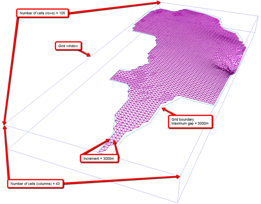
Example showing the grid window, boundary and resolution

Gridding algorithms

A gridding algorithm consists in principle of two main steps:

1. Sorting the input data into a sort grid for fast retrieval in next step
2. Applying an interpolator for interpolating input data into grid nodes

Sorting input data
If the gridding algorithm uses all the input data when evaluating a grid node it is called a global interpolator. This is applicable for minor datasets. For large datasets there has to be a sort step selecting a local set of points around a grid node to be evaluated.

When millions of points are input, the sorting step plays an important role for fast sorting and retrieval of points into the interpolator. An underlaying fine sort grid will hold the indices of the input points thus keeping the original xyz positions. Sometimes several input points may share the same sort node which results in a mean value.

When the interpolator needs input points to evaluate a grid node, it starts a spiral search in the sort grid looking for points. The spiral search works until one of the following criteria is satisfied:

1. Points found in a sufficient number of sectors have been completed.
2. The sufficient number of total points are collected.
3. The max number of spiral searches are reached.

Interpolation
The interpolator is a mathematical function that evaluates a grid node from input data in the nearby region of that grid node. The algorithm can try to honour every data (thru interpolation) or it can produce a surface that is approximating the data producing a smoother surface in regions with very noisy data. Even with an interpolating algorithm, there will be some approximation when the density of the input points are higher than the resolution of grid nodes.

The grid nodes are the data carrier for the input points and if a dense set of input points are to be honoured in the grid, the resolution of the grid must correspond.

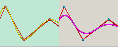
Example of functions controlling interpolation and approximation between data points

When the search procedure is completed the points are submitted to the interpolator and the grid node is evaluated.

Geocap has many different gridding algorithms to choose between. Each algorithm will look at the input data in different ways when deciding what values to give the different grid cells. Below is a list of the different gridding algorithms in Geocap with a short explanation of how they work.

Parabolic

This interpolator generates values into each grid cell, using a parabolic function. For each grid node the interpolator collects the nearest input data and tries to fit a parabolic surface trough them. The xy position of the grid node in the parabolic surface gives the value of the grid node. The interpolator produces local extremal values that can be different from the input data. This tends to create a smooth and "geological pleasant" surface. The interpolator can handle fault lines by setting up blocking areas in data collection to a grid node.

Moving average

This interpolator uses a weighted-distance formula that averages the heights of the input points as the interpolator moves away from the grid node. Local extremal values will always be at the input points.

Blending (parabolic + moving average)

The Blending interpolator blends the properties from the Parabolic and Moving Average procedures in a heuristic way. It uses moving average when only a few points are collected and blends parabolic and moving average for many collected points.

Surfit

The surfit algorithm is based on CMOFS (consecutive minimization of functionals sequence) described on the Surfit home page. The CMOFS algorithm has good qualities handling interpolation and extrapolation. The resulting surface can be comparable with a surface created by Kriging or Minimum curvature method.

Snapping to grid nodes

The snapping algorithm puts data directly into nearest grid node positions of the input data. The following options are available:

• Snapping to one grid node. - The nearest grid node gets the data point.
• Snapping to three grid nodes. - Three nearest nodes of the grid cell that holds an input point get the data point.
• Snapping to four grid nodes. - All four nodes of the grid cell that holds an input point get the data point.
• Snapping to nine nodes. - The nine node snapping algorithm puts data directly into the nine nearest grid nodes closest to an input point.
• Auto find grid. - This method is a one node snapping algorithm. It should only be used for datasets that already is in a grid form. The algorithm will automatically find the grid increments in x and y direction so there is no need for specifying grid increments.

If a grid node is already occupied, mean values will be calculated. Snapping is the best gridding algorithm for dense dataset where the positions of the original data more or less correspond to the position of the grid nodes.

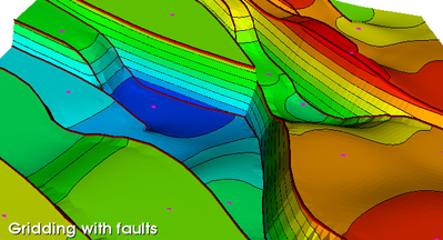
Gridding with faults

The parabolic and moving average interpolator can handle fault traces as secondary input to control the gridding. Only points visible from a grid node to be evaluated will be submitted to the interpolator. Three types of faults traces can be handled:

1. Single fault traces, also called stick faults with no z values and single lines to represent faults.
2. Closed faults traces with no z values representing xy position of upper and lower fault locations.
3. Closed fault traces with z values representing exact position in xyz of upper and lower fault locations.

Use the menu Gridding points, lines and faults to grid points or lines in combination with faults.

Gridding with trends

A trend grid can influence the gridding: The user can specify the influence of the trend grid as a factor when gridding. Trend gridding is used when there is an underlying trend that shall be reflected to some extent in the gridding result.

Line gridding

A line gridding algorithm sees the lines as the data carrier. The gridding mesh is established by making cut points in both directions with the input lines. The cutting process can apply linear interpolation or use spline under tension to get a curved interpolation. Line gridding is applied in the menu Gridding of theoretical profiles.

Triangulation

Triangulation is an option when making a data surface. It is seldom used as the final surface representation, but it is used as an intermediate step in the fault gridding algorithm to honour the fault traces.

Examples of grid algorithms

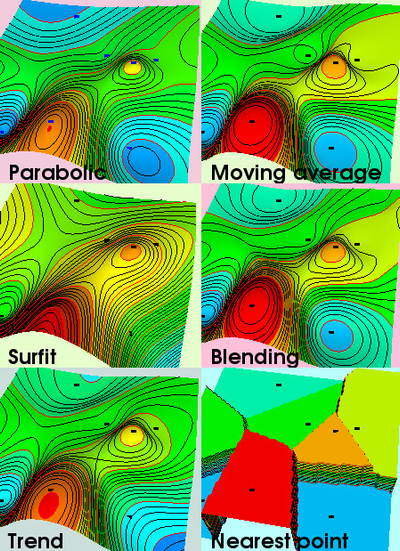
Various grid algorithms for the same input points

Gridding points with fault traces as input

Interpreted seismic lines and fault traces

Linear gridding of theoretical profiles

Gridding commands

Input to gridding are polydata which means points and lines in various forms. For polydata the following Gridding commands are present:

Border model gridding of closed lines

Will make a reference grid or mask grid to determine the defined area of a surface.

Cube gridding from spatial points and scalars

Cube gridding to be used for a small or moderate number of points with scalars.

Gridding of theoretical profiles

Input are lines representing trenches or channels. Used in the Seafloor module.

Gridding points and lines

Gridding of free points and surface lines. Many parameters to control the gridding.

Gridding points, lines and faults

Same as above with additional option for fault lines and trend grids.

Nearest node gridding

Snap node gridding to one, three, four or nine nearest nodes.

Simple points and lines gridding

Easy gridding menu for points and lines ranging from well data to multibeam sonar data.

There is another gridding menu present in Seafloor using multiple charts covering and area or along a line. A single chart represents a grid window for that area and will select corresponding data. Seafloor users and Shelf users have access to that gridding menu which is advantageous when there is a need for splitting a large area into many smaller charts. The gridding algorithms concerning point search and interpolation methods are the same as in the main part.

The gridding process

In this section we will use Simple points and lines gridding as an example to explain the fundamental gridding process. Other gridding commands will have the same basic features. Practical gridding is further explained in Case study - Gridding of seismic interpretation data with faults.

The example is taken from a set of interpreted seismic lines, in this case the seabed. The lines go in all direction according to the survey lines.

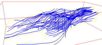
Interpreted seabed survey lines

The gridding command called Simple points and lines gridding indicates that there is only one dataset as input. No extra lines in forms of faults or trend lines are possible. The menu is useful for data points of following input type:

• Single points like well data or scattered data in general.
• Line data where the lines have a dense set of points.
• Single and multi beam sonar data.

The gridding process will normally consists of the following steps:

1. Establish a grid window - Should contain the area of interest.
2. Select a proper resolution - Should have a resolution that honors interesting data.
3. Determine the grid boundary - The defined area covers the area that has input data.
4. Select a proper grid algorithm - A good result depends on a good algorithm.
5. Perform the gridding and check the result. - Perform gridding with various parameters if necessary.

Establish a grid window

The grid window defines the min and max values of the grid. Here are some ways to set the grid window:

• Enter values in the window boxes.
• Click Update from input to get an exact fram around the data line Zoom to Data.
• Click Update window to transfer the present window into the window boxes.

In all cases draw the grid window to visually see the grid frame drawn on the screen.

Select a proper resolution

In this menu the grid resolution is specified by entering the grid increments. The number of grid nodes in rows and columns are automatically calculated this may not be the case on other gridding menus). Keep the overall size of the grid within reasonably limits for practical purposes, f.inst. lower that 3-4M nodes for standard PC's. Also apply Adjust increment which will adjust the grid window values to be on integer grid increment bounds.

Determine the grid boundary

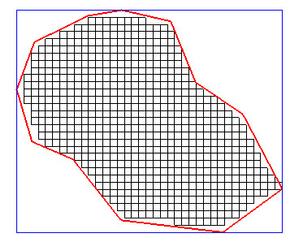
A closed boundary (or border) line defines the area inside within the grid window limits, to be the defined area of the grid. One can use a reference grid or a boundary line that can be digitized or automatically generated. Try various values for maximum gap and push Check boundary to see the result until pleased.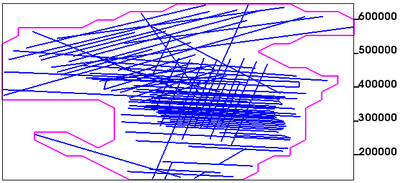

Automatic generated border line
The axes notation to the right indicates the distances in the grid and the maximum gap value.

Select a proper grid algorithm

The main interpolator is parabolic which make a geolocically nice surface. This interpolator is trend sensitive and one should try to use two gridding steps with the surfit interpolator which creates auxillary points in open areas where little or no input points are present. The auxillary points are also saved in workspace as ggg_aux_points during the gridding process.

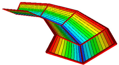
Perform gridding and check the result

The result grid is written back into the project. It is a matter of taste to apply smoothing to the grid result because it can anyway be done afterwards.

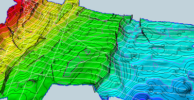
The color band display is produced with General Display with a suitable setup and the input lines were displayed on top. The interpolator secures that the surface will honour the input points. The smoothing will remove noise from the grid and absolute honouring may vanish. Be aware that inherit noise in input data, for instance from auto tracking, may better be removed on beforehand by the spike filter.

The gridding is usually fast and it may be practical to perform several griddings with different parameters to learn and see how the result best can be achieved.

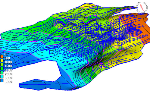
Grid result shown as color bands and input lines

Reference grid

A reference grid is a grid that tells where the defined area of a grid shall be. The reference grid is created by a closed polygon and gridded by the menu Border model gridding of closed lines or gridded directly in the selected gridding menu.

A reference grid can also be generated automatically. That is described in 6. Gridding#Determine the defined area.

The z values of the reference grid are zero. Then one can add the reference grid to any structure grid with the same grid size and get the intersecting surface result. Thus the reference grid serves as a mask grid.

Reference grid created from a closed polygon

Smoothing a grid

The information content of a grid lays in the grid nodes. The grid can have details like sharp fault areas or correct modeled tops and bottoms. But a grid may also have inherent noise in its grid nodes. To get rid of the noise the grid can be smoothed. The noise represents details that should not be there. Thus it is unwanted information.

Smoothing by eliminating grid nodes

This is the standard smoothing method for grids and is used in many menus when smoothing is an option. It is f.inst. used in gridding procedures and in Gradient band analysis.

A controlled way of smoothing is to use the command grp exc

        # regridding grid in active to get rid of noise
        ssc ; # self scale to establish grid window
        grp exc ; # eliminating grid node to be evaluated

grp exc will regrid the grid, but will keep the same resolution. For each grid node a 3x3 grid node pattern is set up. The smoothing effect is achieved by excluding the grid node to be evaluated so that only the 8 remaining grid nodes are input to evaluate the grid node using the parabolic interpolator as default.
When a grid node is recalculated from its surrounding grid nodes the noise in the grid node to be evaluated will disappear because that information is not present in the surrounding grid nodes.

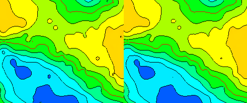
Result of smoothing by excluding a grid node using grp exc

Smoothing by regridding

A simple and direct way to reduce information in a grid is to regrid to a coarser grid so there are fewer grid nodes to hold the information. This can be demonstrated with this little code example.

        # regridding grid in active to get rid of noise
        ssc ; # self scale to establish grid window
        grp sav ; # save grid resolution
        grp long 70 ; # regrid to 70 nodes on the long side
        grp ret ; # return to original resolution

One can regrid to a courser resolution when no specific concern is to be taken. The sampling to new grid nodes is somewhat random and the result grid is smoother.

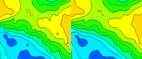
Result of simple smoothing by regridding to a coarser resolution

Smoothing using a menu

To smooth a grid and possibly avoid fault areas or selected points.

This menu will smooth a grid using the special smooth interpolator grp exc. The menu can optionally control point areas, fault lines or closed regions where smoothing is not allowed.

To smooth a grid containing faults it is most efficient to apply a border model grid of the fault traces as input. Apply the check box for smoothing options and select Smooth outside lines or grid areas.

To smooth a surface, but not on specific tops and bottoms, digitize points for these locations and save in a file. Then apply the check box for smoothing option and select Smooth outside single points.

Saving the various smooth steps into workspace will give information about the different smoothed grid. Looking at them, one can decide the best grid to apply.

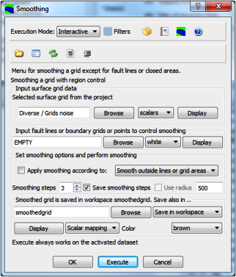
Menu for smoothing a grid

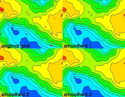
Result of several smoothing steps using the smoothing menu

Rotated grids ^(Geocap8)

Geocap8 supports display of rotated grids and cubes. Many commands related to gridding and grid handling also supports rotation. These include

• grp (gridding)
• grp sav
• grp ret
• bmo (gridding)
• zap
• mak fre
• mak p
• mak g
• pro
• gr3