4. Gridding survey data
- Tore Sannes (Unlicensed)
- Erlend Kvinnesland
- Harald Sund (Unlicensed)
In this section: This command will do the gridding (terrain modelling) of selected points inside the defined area. The result is a terrain model (DTM), which in Geocap will have a schema of type Structured Points. The command will appear as 4 different names, dependant on the folder schema type it is executed from. The commands are: Gridding: Executed from a folder of schema type Generic. Gridding Chart: Executed from a folder of schema type Charts. Gridding Files: Executed from folders of schema type Soundings or Single Beam. Gridding Multibeam Data: Executed from folders of schema type Multibeam. The upper part of the menu contains the project name and the name of the active folder of type Generic, Charts, Soundings, Single Beam or Multibeam. Then the menu contains the parts: The lower part of the menu contains the standard Geocap buttons: The Execute button will execute the selected method, the OK button will save the parameters in the menu and close the menu, and the Cancel button will close the menu without saving the parameters. Set parameters for how the terrain modelling should be executed. Parameters in the Gridding part. The Gridding Algorithm is the selection of the method for the gridding: The X increment (m) and the Y increment (m) are the definitions of the grid cell size. Use Yinc=Xinc means that the value of the Y increment should be the same as the X increment. Use Automatic increments means that the command itself will calculate the X and Y increments. Automatic scale means the minimum and maximum of the data area should be taken from the input datasets. (This option is not available in the Gridding Charts command.) Scale to specified dataset means that the minimum and maximum of the data area should be taken from the dataset which is browsed in below. The dataset can be browsed in from the project. (This option is not available in the Gridding Charts command.) Use increments from grid means that if the specified dataset is a grid, also the grid increments will be taken from the grid. (This option is not available in the Gridding Charts command.) Use Boundary Polygon means that the DTM area should be inside the specified boundary polygon. The Polygon can be browsed in from the project. For the Gridding Charts command the polygon is saved as Boundary in the chart folder. Automatically Create Boundary Polygon means that the boundary polygon will be be created around the input data. The name of the polygon will be Boundary, and for Generic type of folders several versions can be created. Use Hole Polygons means that the DTM area should not be defined be inside the specified hole polygons. The polygons data set can be browsed in from the project. For the Gridding Charts command the polygon is saved as Holes in the chart folder. Use Coastline Polygons means that the DTM area should not be defined be inside the specified coastline polygons. The polygons data set can be browsed in from the project, also for the Gridding Charts command. Ahead of the tabs there are two buttons for using the filtering and smoothing options: This is a new algorithm implemented in Geocap 6.5. It is using a spiral search around each node and honours all input points. This algorithm is built for parallel processing (using several cpus). The parameters for the Parabolic algorithm. The search for points for a grid node. The figure above shows the concept of the point selection. The actual grid node to estimate is in the middle of the grid raster. In the figure above the search radius set to 3. The interpolator will start with collecting the points from the closest cells, marked as Search 1 in the figure. If the requirements for Minimum number of points, Minimum number of quadrants and Minimum points in quadrant are fulfilled, the collected points are sent to the parabolic interpolation algorithm. If not, the interpolator will collect all the points within the Search 2 area, and if necessary continue with the Search 3 area. If the requirements for the number of collected points are not fulfilled, the node will remain undefined. When calculating the depth value in the grid node, the parabolic interpolator will be used: Z = ax2 + by2 + cxy + dx + ey + f This is an algoritm which reads input points and distribute the weighted values into the grid nodes. This method can read an unlimited number of points and files. The limitation will be on the size of the individual files and the result grid. The parameters for the Weighted Average algorithm. Search radius is the maximum distance in for distribution of points around a grid node. The value is multiples of grid cells or as a metric value. Weight function. The weight can be calculated as a linear or a square value dependant on the distance from the node. Specification of the weight function: If the distance from the grid node to the point is small, the minimum distance is set to 1% of the grid increment. The search for points for a grid node. The figure above shows the concept of the point selection. The actual grid node to calculate is in the middle of the grid raster. In the figure above the search radius set to 2 grid nodes. All the points within the search radius are snapped to the grid node when reading the points. For each node the sums of distance * weight and the sums of the weights are calculated for each snapped point. After reading all points from all datasets the node value is calculated by dividing the sum of distance * weight with the sum of the weights for every node. The algorithm is good for scattered points like polygon data or single beam data. It should not be used on large amounts of data from for instance multibeam echo sounders. The parameters for the Multilevel B-Spline algorithm. The Multilevel B-Spline interpolation grid structure for levels 0 and 3. The maximum level is 14. When all the interpolation iterations are finished, the final grid is extracted from the cubic B splines by looking up the depth value in the positions of the final grid nodes, given by the width and height and the specified grid increments. The binning algorithm collect the points closest to each node and calculates one or several values. When executed on a folder of type Generic (not Charts), several types can be created in one run. The parameters for the Statistical binning algorithm for Gridding (left) and Gridding Charts (right). Minimum number of points in cell: If the cell has less points than the minimum, the cell will not be defined in the result grid. The point selection for the Statistical binning algorithm. The figure above shows the concept of the point selection. The actual grid node to calculate is in the middle of the grid raster. All the points within the grid cell size are snapped to the grid node when reading the points. For each node the value of the minimum and/or maximum value is updated for each new point. For calculating the mean and standard deviation values, the sum of the depth values and the number of points in each cell is kept. For calculating the standard deviation, the input points are read once more to calculate the sum of squared differences for all points versus the mean value in the grid cell. Variance = Sum_of_squared_differences / (number_of_points-1) When checking the parameter Filter input points a filtering process is applied on the input data. The filter process will do two times gridding using the same algorithm. Between the two gridding sequences a filter will be run on the input data. The filter is calculating the deviation between each point and the initial (first) grid, and the points within the limits of the filter is accepted. The accepted points will be used in the second gridding. The parameters for Filter and re-grid. Save filtered points: Save the accepted points as Soundings_Accepted and the removed points as Soundings_Rejected. Filter type: Use deep limit=shallow: Use the same limit on both the shallow and deep side of the initial grid. Shallow factor: Factor for multiplying the calculated standard deviation as limit on the shallow side of the initial terrain model. Deep factor: Factor for multiplying the calculated standard deviation as limit on the deep side of the initial terrain model. When checking the parameter Apply smoothing, a smoothing process is applied on the output grid. The parameters for Smoothing. Smoothing method: Filter width: The size of the filter mask. The node to be smoothed is the one in the middle of the mask. Filter weight: Parameter used by the Convolution method. The value is the sum of the weights for the ponts in the mask. The point to be smoothed gets the weight 1- filter weight. This part is visible for the commands Gridding, Gridding Files and Gridding Multibeam Data. Select in the list which files to do gridding on. The area for the DTM is taken from the extension of the input files. The corner points are justified to fit the selected increments. This part is visible for the command Gridding Chart only. Select in the list for which charts to do gridding. The area for the DTM is taken from the chart definition, and the input data is the Soundings data set. Also the Boundary and Holes data set might be involved. After executing the gridding a dialog will pop up showing the parameters, result and statistics from the gridding. The report itself is saved in the project structure in e folder named Reports located under the actual folder. The report itself is named as YYYYMMDD Gridding (or the name of the actual executed gridding command).Introduction
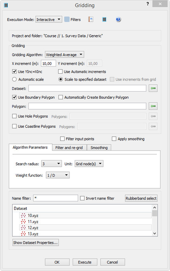
The content of the menu
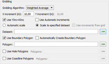
The parameters for the Gridding part
The parameters for the Tab part
The Algorithm Parameters tab
The Parabolic algorithm
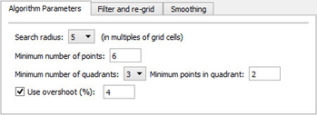
Search radius is the maximum distance in for collection points around a grid node. The value is multiples of grid cells.
Minimum number of points is the minimum number of points totally for estimating the grid node.
Minimum number of quadrants is the minimum number of quadrants around the node which contains at least a specfied number of points.
Minimum points in quadrant is the minimum number points in a quadrant to estimate the node.
Use overshoot (%) is a parameter which controls the mathematical calculation of the grid node.
For each node the Zdiff=Zmax-Zmin from the collected points is calculated. The value dZ is calculated by dZ=Zdiff*overshoot(%). The resulting Z value will be within Zmin-dZ and Zmax+dZ.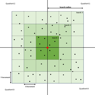
The Weighted Average algorithm
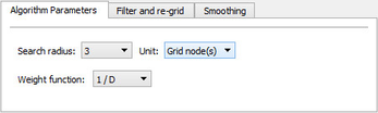
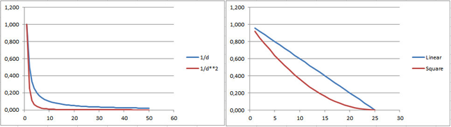
The weight functions for search radius 25.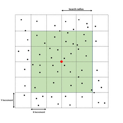
The Multilevel B-Spline algorithm
The algorithm interpolates scattered points by a tensor product of uniform cubic B splines on a m0 x n0 grid. The start level (0) is 1x1. The grid is refined to size (1x2i+3)x(1x2i+3), where 'i' is the current number level. The algorithm stops refining the grid when the RMS error over points is greater or equal Max RMS error or the level has reached Max levels.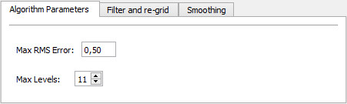
Max RMS error is the maximum allowed error for the points versus the grid.
Max levels: The maximum allowed levels of refining the grid. In the Gridding command the value can not be larger than 14. This level work with a refined grid of size 268,5 million nodes (16378x16378).
The Statistical Binning algorithm
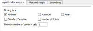
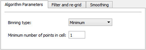
Binning type is the method for calculating the grid node: 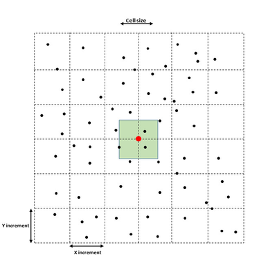
Standard deviation = Sqrt(Variance)The Filter and re-grid tab
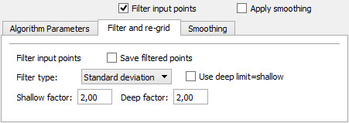
Calculate the standard deviation from all input points versus the initial grid. The standard deviation is multiplied with the shallow factor and \n the deep factor to get the filter limits.
The depth are filtered by absolute distance from the initial grid.
For each point, get the depth from the initial grid. Calculate the shallow and deep limits by multiplying the % value limit with the depth.The Smoothing tab
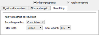
The center node is getting the weight 1-filter weight, while the rest of the nodes gets the weight filter weight/n-1, combined with a distance weight. The center node value is the weighted average of the depths in the filter.
The median filter is a sorted list of depth values of the nodes in the filter, while the centre node is getting the median value of the sorted list.The parameters for the Dataset part
The resulting DTM will be saved with the name Surface_<algorithm name> in the current folder. Several versions kan be saved as Surface_<algorithm name> (n) in the same folder.The parameters for the Chart Name part
The resulting DTM will be saved with the name Seafloor. Only one Seafloor will be saved in a chart folder.The Report