Reading and visualizing seismics
- Anders Moe
Reading SEG-Y Files
Analyzing a SEG-Y file
When reading SEG-Y files consider whether to use default settings or if the particular file in question requires a separate analysis pre-step. By performing an initial scan of the file you can provide layout parameters to the reader tools. See Analyzing SEG-Y files for a detailed explanation on how to analyse SEG-Y files.
How SEG-Y files are converted
All SEG-Y tools will read a SEG-Y file and output a feature in a feature class corresponding to the navigation geometry. The seismic data (ie the amplitudes) are output in a separate file and referenced in the feature using the url field.
Reading SEG-Y 2D data
If the SEG-Y file requires a separate prescan in order to determine the layout, please consult the section Analyzing SEG-Y files. Skip this to use default values.
To read SEG-Y 2D data:
- Open the tool Read SEG-Y 2D files.
- In the first entry, select one or more SEG-Y 2D files.
- Click on each field to see the documentation shown on the right.
- Click OK to begin reading the SEG-Y file(s). Each file will be appear as a feature in the target feature class.
See Visualizing Seismics to view the seismic data.
Reading a SEG-Y 3D outline
You can use the tool Read Outline from SEG-Y 3D File to read the outline of a seismic 3D survey in one of three ways:
- As a plain rectangular bounding box. This rectangle will in general include some areas without real data.
- As an outline without null traces (missing traces)
- As an outline without null traces and zero traces (traces with only zeros)
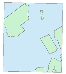
The above figure shows two readings. The blue area is the result of reading the outline as a plain boundary. The green areas are the true data coverage created when skipping the empty traces and the zero-traces. As is evident there is a significant discrepancy.
Consider using this tool to create accurate survey outlines.
If the SEG-Y file requires a separate prescan in order to determine the layout, please consult the section Analyzing SEG-Y files. Skip this to use default values.
To read a SEG-Y 3D outline:
- Open the tool Read Outline from SEG-Y 3D File
- In the field SEG-Y File enter the SEG-Y file that you wish to import.
- If required choose a SEG-Y Settings file created using the SEG-Y Analysis dialog. If you omit this step default settings will be used.
- In the field Feature Class Source choose whether to create a new seismic feature class or use an existing one.The seismic feature class will contain metadata for the SEG-Y file.
- Depending on your previous choice, select an existing seismic feature class or enter the location and name of a new one.
- Choose coordinate system. This is not required but is generally recommended.
- In the field Outline Type choose one of the following:
- Basic Rectangle. Effectively the bounding box enclosing the outer perimeter of the survey. The quickest solution.
- Without null traces. Skips missing traces.
- Without null and zero traces. Skips missing traces and traces containing only zeros. This leaves only valid data and should be your choice if you whish to extract an exact coverage.
- Click OK. This will begin the reading of the SEG-Y file and creating the outline feature in the selected feature class.
See Visualizing Seismics to view the outline.
Reading SEG-Y 3D data
If the SEG-Y file requires a separate prescan in order to determine the layout, please consult the section Analyzing SEG-Y files. Skip this to use default values.
To read SEG-Y 3D data:
- Open the tool Read SEG-Y 3D File
- In the field SEG-Y File enter the SEG-Y file that you wish to import.
- If required choose a SEG-Y Settings file created using the SEG-Y Analysis dialog. If you omit this step default settings will be used.
- In the field Feature Class Source choose whether to create a new seismic feature class or use an existing one.The seismic feature class will contain metadata for the SEG-Y file.
- Depending on your previous choice, select an existing seismic feature class or enter the location and name of a new one.
- In the field Output File Format select format for the output data file. We recommend that you stick to the default Raster that also creates statistics and pyramids. Learn more about these formats in the section Seismic output formats.
- Enter the location for the output file (s). This will be the directory for the seismic data files. The tool will create a subdirectory in this folder.
- The checkbox Store paths relative to the geodatabase lets you choose whether the seismic feature class will store absolute or relative paths to the seismic data. Choose relative if you expect to move the geodatabase along with the seismic data to a different file location. It is generally not required to check this options, since you can use the tool Set Seismic URL to reset the URL to a new storage location.
- In the section Z-domain choose depth or time along with a unit, depending on what is appropriate for your seismics. The domain type will be stored in the seismic feature class. No depth conversion will take place.
- Click OK. This will begin the reading of the SEG-Y file, adding the outline and metadata to the seismic feature class and creating either a separate brick file or an index file.
If you created a new seismic feature class during the reading of the SEG-Y file you may need to refresh the geodatabase for the feature class to become visible.
See Visualizing Seismics to view the seismic data.
Creating a seismic feature class
Seismic feature classes can be created as a separate step, not necessarily as part of the SEG-Y import. You will create different seismic feature classes for 2D or 3D as well as for 3D survey outline.
To create a seismic feature class:
- Open the tool Create Seismic Feature Class. The dialog for this tool will appear.
- In the field Output Location select the target geodatabase that will store the feature class.
- In the field Feature Class Type enter one of the following:
- Seismic Lines - for reading SEG-Y 2D files.
- Seismic Cubes - for reading SEG-Y 3D files.
- Seismic Cube Outlines - for reading 3D survey outlines.
- Enter the name of the feature class to be created.
- Enter the coordinate system.
- Click OK. The feature class will be created in the geodatabase.
You may need to refresh the geodatabase for the newly created feature class to become visible.
Visualizing Seismics
This section describes the various interaction modes available when visualizing seismics.
Regardless of method you should always ensure that your 3D window is aligned to the spatial positioning of the seismics.
To align the 3D window:
- Locate the 3D Explorer toolbar :
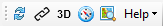 . If needed create the 3D window by clicking the 3D toolbutton.
 - In the 3D Explorer toolbar click the Zoom to Map toolbutton :
 . This will align the 3D view to the 2D camera position.
General Viewing
To visualize seismic outlines:
- Add the seismic feature class to your table of contents. Turn it on. This will display the seismic survey geometry in the 2D data view.
- The seismic outline should automatically appear in the 3D window. If not perform the alignment steps described earlier in this section.
To visualize a 3D cube:
- Add the feature class containing your seismic 3D surveys to the table of contents. Turn it on. This will display the seismic surveys outlines. The seismic outline should automatically appear in the 3D window. If not perform the alignment steps described earlier in this section.
- In the map or table of contents, use the built-in ArcMap selection mechanism to select the survey that you wish to view.
- In the seismic toolbar click the button
 . This will display the seismic cube in the 3D window.
 - To move sections in the 3D window: In the 3D window use Shift + Left mouse button to drag the seismic sections.
- To move sections in the 2D map view: In the seismic toolbar click the button
 . On the map, click and drag the inline or crossline that you wish to move. The section will move in the 3D window as well.
To visualize 2D seismics:
- Add the feature class containing your seismic 2D surveys to the table of contents. Turn it on. This will display the surveys lines. They should automatically appear in the 3D window. If not perform the alignment steps described earlier in this section.
- In the map or table of contents, use the built-in ArcMap selection mechanism to select the survey that you wish to view.
- In the seismic toolbar click the button . This will display the seismic lines in the 3D window.
Viewing particular sections
In general you may have several 3D surveys displayed. This will populate your table of contents with several cubes giving you a choice of which sections to view. Here we will describe how to make ArcMap operate on a particular section.
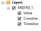
A cube dataset looks like this in the table of contents:
To activate and view a seismic section:
- Ensure that the 3D cube is visualized as described earlier in this section.
- Locate the cube dataset layer in the table of contents. This dataset will contain the cubes inline, crossline and timeslice.
- In the cube dataset click the inline, crossline or timeslice object.
- In the seismic toolbar click the button
 to activate the highlighted section.
 - In the 3D window press the shift button while dragging the corresponding section with the mouse.
The seismic toolbar will display the active section along with the section number. You can use the arrow buttons to move the section.
Color Ramps
Seismics are colored using one of the color ramps available as part of the Seismic Explorer distribution. This section describes how to apply different color ramps.
To apply color ramps:
- Start out by displaying your seismic data as described in the section on visualizing seismics.
- In the seismic toolbar locate the color ramp selector :

- Click on the small arrow on the right side of the control to select one of the available color ramps. This is now the current color ramp and will be applied to subsequent renderings.
- The seismic will be re-rendered according to the selected color ramp.
Often the data range exceeds the range that you want to color. This may be caused by noise in the extreme ends of the data range, for example. In this case you want to narrow the data range that is being mapped to the color ramp. By default color ramps are zero-centered. However you can adjust the color mapping asymmetrically.
To adjust the data range for the color ramp:
- In the color ramp selector drag one of the handles positioned on the current color ramp while holding down the left mouse button. This will symmetrically increase or decrease the data range being color mapped.
- As an alternative, drag the handles using the right-mouse button. This will move only one of the sliders. Use this to adjust only the top or bottom of the data range. This is useful for data that is not zero-centered.
You can reverse a color ramp by clicking  .
.
Performance tip
To improve the display performance when viewing seismic sections consider turning off the layers for sections that you do not wish to view
Seismic output formats
When importing seismic 3D cubes you have a choice of output formats. Each option has some advantages and disadvantages.
Raster files.
- This is the recommended output format, supported since version 2.3.4
- This format converts the seismics to ArcGIS rasters for maximum performance.
- Require if you wish to publish the seismics later to Seismic Server.
- If using full 32 float output the resulting rasters may be almost three times the size of the original. If using 16 bit or 8 bit the raster may be comparable in size to the SEG-Y file or even smaller. The exact output size will depend on how successfully data regions like water and undefined values are compressed.
Index file:
- An index file is a compressed index into the original SEG-Y file. It is used to quickly access parts of the SEG-Y file. Data is therefore read from the original file. The index file itself contains no data.
- Index files are small. Even SEG-Y files hundreds of gigabytes in size result in index files that are only a few hundred kilobytes in size.
- When you create an index file the Geocap Seismic Explorer will use the index file during visualization to read data from the original SEG-Y file.
- Visualization performance when using an index file is acceptable for moderately sized cubes, but will suffer as the cubes increase in size.
- Showing timeslices will always be relatively slower than inlines and crossline display.
Brick file:
- This format is a legacy format and may not be supported in future versions.
- Contains all the data from the original seismic cube. It is essentially a 3D partitioning of the seismic cube stored in a format that optimizes I/O.
- A brick file offers excellent visualization performance for cubes that are many hundreds of gigabytes in size
- A brick file will be somewhat bigger than the original file, typically something like 10% depending on the size of the original SEG-Y file.
- Once the brick file is created the original SEG-Y file is not needed anymore by the Geocap Seismic Explorer.
In short : If visualization performance is important or if you intend to publish to Seismic Server, choose rasters. If preserving disk space is more important than maximum visualization performance, choose index file.