Depth Conversion of time surfaces
- Erlend Kvinnesland
- Former user (Deleted)
- Harald Sund (Unlicensed)
Introduction
This documentation goes through the working steps and menus in Geocap for depth conversion of time surfaces applying a time-velocity cube. There are other methods for depth conversion than those described here, but this method is favorable when stacking velocities and well data are present. This depth conversion documentation deals with quality control and analysis of input data. Then gridding into a time-velocity cube and finally performing depth conversion of time grids in a Layer Model into depth grids.
The velocity cube reflects the information in the velocity data in an organized way. Working with velocity cubes will make depth conversion of time data to depth data more easy.
In this section:
Steps in depth conversion
Steps in depth conversion of time data using time-velocity cube
- Reading stacking velocities into a folder as: x y time velocities
- Inspecting the velocity data
- Gridding into a velocity cube
- Displaying the velocity cube
- Checkshot wells can be used to trim the velocity cube through sophisticated updating techniques
- The velocity cube is then used for depth conversion of time grids into depth grids
- Calculation of cubes for RMS and Interval velocities using the generated velocity cube. (Option)
The folders used to save data in this project are of type Generic and renamed to indicated their contents. The various datasets will also be set to their proper schema type so that only relevant command objects are shown.
The documentation follows a specific dataset and is thus close to a case study. This implies that other dataset may apply slightly different display options due to size and attribute saving in scalar or field data. The general principles for depth conversion should however be the same in all cases when using the method of a velocity cube.
Example of velocity cube holding stacking velocity data
Reading stacking velocities
Geocap provides import command objects (CO) for reading stacking velocities organized in ASCII column data.
If the file is large, keep the input as low as possible. To generate a velocity cube only x y time velocity are needed.
Example input: stacking velocities in ASCII columns, size ~ 400MB.
Reading stacking velocities into a project
- Create a Generic folder, give it a proper name
- Right click on the folder and select *Import->Stacking Velocities.
- Browse in all stacking velocity datasets
- The cell structure is kept by specifying 'Value change' and set up 'cell separator' for the actual column
- The schema type is set to 'Stacking velocities' to get the correct commands visible on the dataset
- In this case the time values are in the z coordinates and the velocity values are scalar values
Geocap project for stacking velocity data and velocity cubes
The actual project was generated the standard way by opening a new project and gradually populate it with folders when needed. The stacking velocities was imported into a generic folder given the name All points in line cells, just to indicate that the stacking velocities are organized as vertical lines, called line cells in Geocap syntax. The schema setting of the dataset is Stacking Velocities.
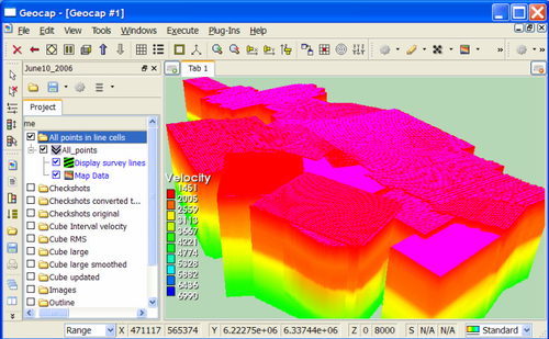
Inspecting the velocity data
The stacking velocity file has nearly 7 million points and there are dedicated COs to make a fast display if necessary like Utilities->Map vertical cells in fast mode. This example applied Map Data and Display survey lines (will only display the top points as lines) to get a visual impression of the different surveys in this dataset.
A closer look at the display shows that it is a collection of many different surveys. The transition between the different surveys may show inconsistencies in velocity data. It is possible and advisable in some cases to adjust surveys to get a better match by standard data manipulation. Gridding stacking velocities into a cube will also smooth out errors and tends to make transitions acceptable.
To display a smaller part of the surveys one can use the CO under Utilities->Display stacking velocities in line mode. Set always the correct attribute (scalar or velocity if field data) and select for example Eliminate outside cursor: A small part of the dataset around the cursor is selected for display and also saved in workspace as elioutcursor. Similar for an area zoomed into when in 2d mode and part of dataset can be saved as workdata in workspace.
Cube gridding from stacking velocities
The command menu Cube gridding from stacking velocities can be activated for data with schema Stacking Velocities. Stacking velocities have the format: x y two_way_time velocity. Two_way_time is used because time is recorded after having traveled down to the reflector and up again.
Set correct attribute for velocity values
Initially, set the correct attribute to tell whether stacking velocities are in scalar or field data velocities or have some other name. Press Set when the correct attribute selection is done.
The cube gridding command menu allows the user to set a proper origin, set the cube increments, use Adjust (gridding window) to Increments to align the cube at increment values. Be sure to set the gridding window correct before gridding. Pressing Window Frame will display the coordinates written in the grid window as a frame. Also check the zmin zmax values to see that the vertical extent is correct.
Expanding the cube grid window
An option that might be useful is to expand the cube gridding window a few grid cells to ensure that the cube is gridded outside the min and max area of the time grids in case the cube gridding window is first taken from the xy window of the time grids. Press Expand to increase the cube gridding window.
When the increments of the cube are correct hit Calculate to get the number of rows, columns and layers in the cube.
Before gridding some options in the grid option page should be set or checked.
The grid option page allows for selecting an outline (or reference line) to determine where the gridding will take place. This is superior to the automatic method.
The Result cube page allows for saving the cube into a folder. A copy is also saved as in workspace as cubegrid. The cube dataset is given the schema Cube. Thus the cube will have many relevant commands visible for further actions.
Testing cube gridding
The Test page in the gridding menu allows for testing the gridding at various cube planes to check the gridding parameters and study the quality of the input. This is done as shown in the display below.
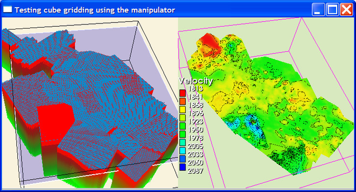
Testing cube gridding using a manipulator plane
After testing the gridding at a few planes and securing all parameters are properly set, the overall gridding of the stacking velocities into a velocity cube can take place. The resulting cube can then be visualized with various display techniques.
Updating the cube with checkshot data
In many cases there are also control data for the velocity cube available in form of checkshot wells. These well data should have the format: x y depth one_way_time. They can be used to update and correlate the velocity cube so that the layers will match the checkshot wells. Use the command menu Utilities->Updating velocity cube to checkshots.
The Set update filter option is available for excluding wells that obviously has wrong starting velocities, namely the sound velocity in water.
Checkshot wells organized in a folder
Sometimes the checkshot wells must be generated by merging velocity and time from one dataset into the well position of another dataset. That is done by the command object Merge x y with two data parameters found under schema type Line folder utilities. Set your folder with well positions to that schema type, or copy the command object from the repository into Item Commands on that folder. Then one can generate the proper checkshot wells from separate well data information.
When reading the checkshot wells into the algorithm, all wells are collected into one dataset. This dataset is also transformed into x y two_way_time velocity so it will match the velocity cube. All checkshot wells are prolonged to go from cube_min to cube_max in order to produce matching data all along the well string. The transformed and prolonged checkshot wells are saved in workspace data as updatedwells and can be further inspected.
The default updating algorithm is called Moving average which means that the differences from the checkshot slice and cube slice are gridded with a moving average interpolator and added to the cube slice.
The Tensor algorithm uses a bell shaped b-spline tensor for updating and is recommended for a local updating around well. A counter for each layer is listed on the terminal window during updating.
After updating the cube with checkshot wells the cube should be displayed and checked that the cube layers are matching the well data.
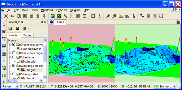
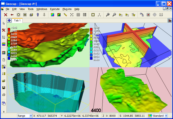
Transformed checkshot wells with bottom layer before and after updating cube
The above figure shows that the cube matches according to the color code of the checkshot wells by displaying the bottom layer before updating the cube (to the left) and after updating the cube (to the right). After smoothing and updating the velocity cube it can now be used for depth conversion.
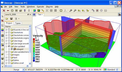
Checking the cube visually
The velocity cube is displayed by dedicated commands available through the Cube schema.
Upper left viewport shows surface contours for the cube using the commands Cube contours.
Upper right shows planes in the cube colored and contoured with velocity using Cube views->Map X Y Z planes at cursor position. That command requires a cursor position inside the cube frame which can be set hitting the keyboard letter p or y while pointing at the screen.
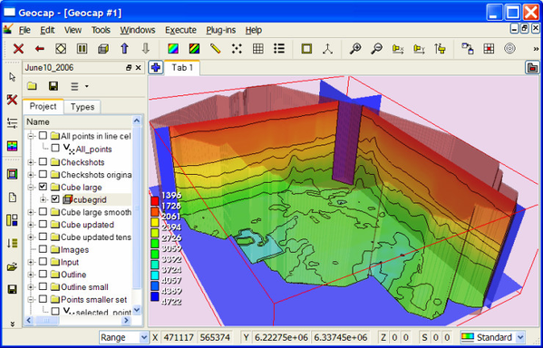
Displaying velocity cube with three planes and transparent surface boundary
Bottom left is a cube overview contoured as a boundary surface using Cube contours.
Bottom right is cube layer at level 4400 displayed as terrain using Display selected cube layers. This menu allows for displaying single cube layers or arranges multiple layers in viewports if this option is checked in on the Viewport display setup page.
Displaying individual layers in a cube is important for checking the cube contents and also for presentation purposes.
Various ways to display cube information
Depth conversion using a dedicated command object
The velocity cube is useful for depth conversion of a set of time grids into depth grids. This formula is used: depth_grid = time_grid x velocity_of_time_grid.
The size of the cube in z direction should be at least a little bit greater than the extent of the top and bottom surface. Also the x y extent should completely include the grid window. Then all the surfaces will fit into the velocity cube.
Requirement
All the time grids should be located in a folder which have the schema Layer Model.
Active the menu command by Layer Model->Depth conversion of time grids in folder using velocity cube.
Read the description on the depth conversion panel thoroughly. Here is a summary.
Fast and convenient method for depth converting all time grids in a folder using a velocity cube
- Set schema of the folder with the time grids to Layer model
- Copy the entire time grid folder to a new folder
- Rename the copied folder to Depth grids. It is still time grids, but will soon be converted to depth grids
- On the folder with depth grids, activate the commands Layer utility > Depth conversion of time grids in folder using velocity cube
- Browse in the velocity cube and hit Execute
- As a result all grids in the folder that were time grids are now converted to depth grid
The central command in depth conversion is the pro command which does the probing of the time grid into the velocity cube. The time grid must be converted to polydata in order have a scalar part: x y time scalar. After probing this dataset into the velocity cube, the scalars are assigned values from the cube at their positions and the whole dataset is now transferred into x y time velocity.
The rest of the procedure is to work out the formula: depth_grid = time_grid x velocity_of_time_grid and saving the converted dataset back into its place.
If by some reason one wants to redo this operation, one has to bring a new fresh set of time grids into a folder and perform the procedure over again.
It is also possible to convert just a single grid from time to depth using the velocity cube. Apply the commands for grids Grid operations->Depth conversion using velocity cube.
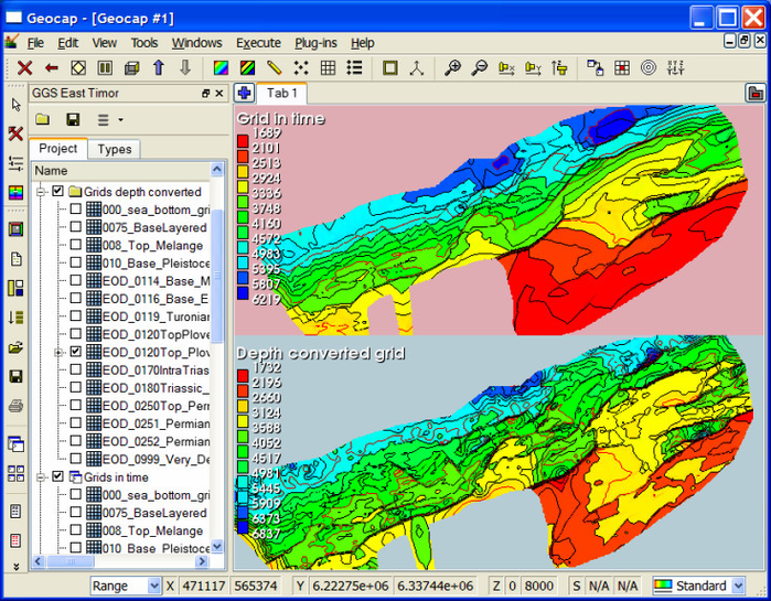
Example of depth conversion from time grid to depth grid
The above picture shows an example of depth conversion a time grid into depth grid using a velocity cube and the same procedure as described above. All grids in the layer model were depth converted simultaneously.
Using base grid datum to minimize cube size
Sometimes the cube spans over a large area going from shallow water near land to deep water far out in the sea. In that case it is suitable to use the seabed as a base grid datum to minimize the cube grid size.
Read more about this feature in the special documentation Time - velocity cube with base grid datum.
Calculations on the time-velocity cube
A time-velocity cube can be smoothed and recalculated to other forms like an RMS (Root Mean Square) or an Interval Velocity cube or even a depth-velocity cube. Read more about these options in Creating RMS cube, Interval cube and Depth-Velocity cube