Volumetric Calculations
- Erlend Kvinnesland
- Former user (Deleted)
- Harald Sund (Unlicensed)
Introduction
Two main approaches for volumetric calculations in Geocap
- Simple volume calculation for maximum two surfaces and two contact planes. To be used in prospect analysis and early stages of a reservoir development. Or for a single grid and a thickness.
- Volume calculation using petrophysical parameters and any number of zones and maximum two contact surfaces (planes or grids). Requires a layer model; i.e. all the horizons are collected in a folder in correct order.
Both cases can handle xy polygon areas that limits the volume calculation to those areas.
In the first simplistic approach, only volumes are calculated for a single reservoir zone or a top structure down to a surface or plane. The petrophysical parameters can only have single values. No petrophysical grids are involved.
In the more advanced, second approach, volumes are calculated for a number of reservoir zones. Each reservoir zone is defined by a top and a base reservoir zone grid, where the base grid of a reservoir zone equals the top of the next reservoir zone. For the reservoir zones, a corresponding set of parameter grids for the petrophysical properties should exist in order to calculate hydrocarbon in place values..
Petrophysical parameters used in volume calculations
- porosity
- water saturation
- net/gross
The parameters may vary laterally across the reservoir, and independently for each reservoir zone. For the specified reservoir, Geocap will report the following volumes:
Reports from volume calculations
- rock volume (the volume between surfaces, optionally within a restricting polygon)
- pore volume (dependent on porosity)
- hydrocarbon pore volume (also dependent on water saturation)
- hydrocarbon in place volume (also dependent on net/gross)
- recoverable hydrocarbon volume (also dependent on expansion (formation) volume factor and recovery factor)
Restricting polygons like license boundaries are supported. Restricting levels like an gas-oil and oil-water contacts are supported.
The volume calculation module has many powerful ways of graphically displaying the reservoir volumes. One example is a horizontal map showing how the reservoir volume changes across a reservoir zone in combination with a cross-section across the reservoir. Another example is reservoir zone volume display. In the picture below the volume of a reservoir zone is shown as a body in three dimensions.
In this section:
Reservoir zone
A reservoir zone is constructed of a top layer and a bottom layer which makes up a volume in between. The difference between the two layers is the isopach. Volume calculation of the isopach will give the volume of the reservoir zone.
Further confinement options of volume calculations
- A top plane (or in general any grid) that will cut through the layers and tell where the volumetric calculation starts.
- A bottom plane (or in general any grid) that will cut through the layers and tell where the volumetric calculation stops.
- Polygon areas that describe the xy extent of the volumetric calculation.
There is also a short training session at Volumetric calculations that can be visited after having read the documentation.
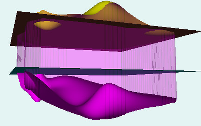
Reservoir zone volume model with top and bottom surface and two contact planes
Simple Volume Calculations
For simple bulk volume calculations the user typically has one or two grids that are to be involved in the volume calculations. The grids are normally in meters and the bulk result will be in cubic meter. But in general all calculations are done in the units of the data. If restricting polygons are to be involved in the calculations, for instance a license boundary, those must also be predefined and present in the project manager.
Simple Volume Calculations requirements: One or two grids in the project manager, and if relevant, restricting polygon(s) and contact planes. Optionally petrophysical parameter values as single values.
The grids can in principle be located anywhere in the project, but it is common to place them inside a Layer Model folder.
Simple bulk volume calculation is much used in prospect analysis and generally to get a quick answer to bulk volume contents. Follow the procedure below for simple volume calculation
Procedure for simple volume calculation
- Right click on the upper grid and select Grid Operations->Volume calculation
- Specify Type of volume to be calculated
- Browse in the second grid if required
- Browse in the restricting polygon if necessary
- Set the contact levels restricting the calculations
- Specify petrophysical values if necessary
- Press Execute to perform the volume calculation
.
Menu for simple volume calculation
Reservoir Volume Calculations
In general a reservoir is made up of multiple layers and zones. These layers are then cut by contact planes or grids to further confine the volumetric calculation. The terms layer and horizon area synonymous and used interchangeably.
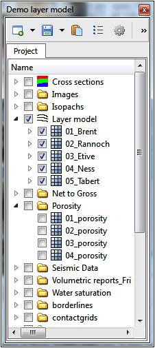
Calculations of multilayer reservoir volumes requires a Layer Model. Create a standard Generic folder and place all horizons into the folder in a correct order; i.e. the top reservoir horizon shall be the first; the bottom horizon is the last. This is most easy achieved by using a prefix on the horizon names: 01_.., o2_.., etc. Finally set the schema for the Generic folder to Layer Model.
- The Layer Model concept is an easy and natural way to set up a multilayer reservoir.
- The zones of the reservoir are between the layers.
- The number of zones are one less than the number of layers.
- The number of petrophysical grids in a generic folder are the same as the number of zones.
- For convenience, the name of a zone has the same name as the top horizon of that zone.
All the petrophysical parameters are corresponding grids to the horizons and resides in separate folders.
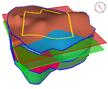
Multilayer reservoir with two contact planes and a license area
Project used in reservoir volume calculation
To calculate the volumes of a reservoir
Procedure for performing volume calculation.
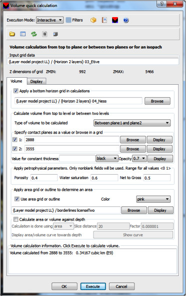
1. Right click on the Layer model and activate Utilities > Volume layer model calculation as shown to the right.
2. Set all parameters correct. In this example we have selected the following parameters:
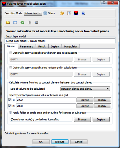
Settings in the *Volume* page
- A gas oil contact plane 1 at depth 2222.
- An oil water contact plane 2 at depth 2888.
- Type of volume to be calculated is set to Between plane1 and plane2.
- A single outline for a license area is applied to confine the volumes.
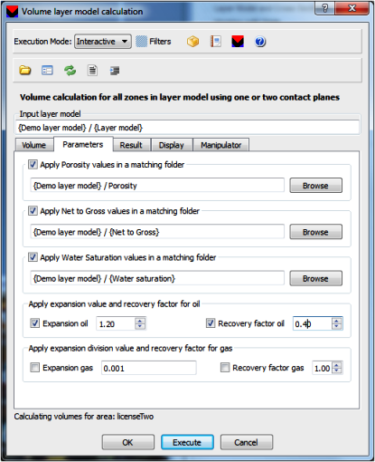
Settings in the *Parameters* page
- Porosity folder is browsed in.
- Net to Gross folder is browsed in.
- Water saturation folder is browsed in.
- Expansion factor for oil.
- Recovery factor for oil.
Important options in volume parameter settings
- Specify correctly the part of the reservoir to perform calculation upon:
- From top to plane 1. Gas is assumed unless expansion value for gas is off and expansion value for oil is on.
- Between plane 1 and plane 2. Oil is assumed.
- A contact entry can be a single value or one can browse in a grid.
3. Click Execute for performing the volume calculation.
4. Go to the Result page to see the results as shown below.
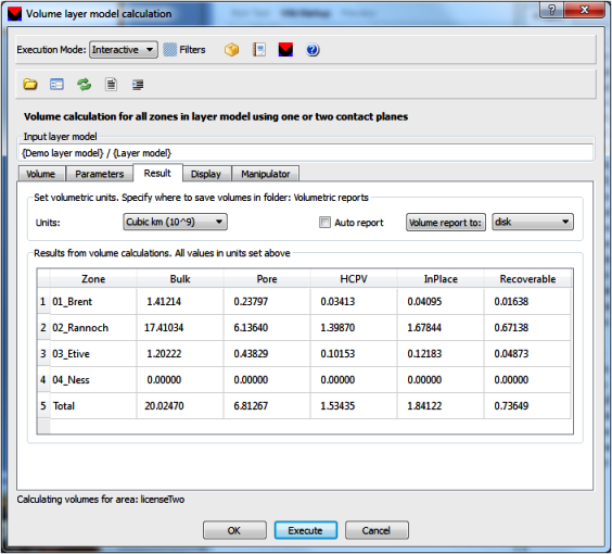
Result menu for volume calculation of a multilayer reservoir model
Front menu for volume calculation of a multilayer reservoir model
An options is to specify another start layer and stop layer for the volume calculation. That is not done in this example.
Below is the settings for the petrophysical parameter grids. If no petrophysical parameters, leave this page blank. Then only bulk volume will be calculated.
Menu page for setting pertrophysical parameters in a multilayer reservoir model
Volume report
The result page has a button for writing a volume report to disk or optionally also to a folder in the project. If Auto report is On, the volume report will be written when Execute is performed.
Project: Demo layer model
Volumetric report for horizons in folder: Layer model.
Calculated and saved at: Tue Nov 15 07_19_08 2011

Parameters present and used:
Type of volume to be calculated: Between plane1 and plane2
First horizon used: 01_Brent
Last horizon used: 05_Tabert

Contact plane 1: 2222
Contact plane 2: 2888

License or sub area: licenseTwo

Porosity folder: Porosity
Net to Gross folder: Net to Gross
Water saturation folder: Water saturation

Expansion value oil: 1.2
Recovery factor oil: 0.4

Units used in report table: Cubic km (10^9)

 Zone                 Bulk           Pore           HCPV           InPlace        Recoverable
 01_Brent             1.412140       0.237970       0.034130       0.040950       0.016380
 02_Rannoch           17.410340      6.136400       1.398700       1.678440       0.671380
 03_Etive             1.202220       0.438290       0.101530       0.121830       0.048730
 04_Ness              0.000000       0.000000       0.000000       0.000000       0.000000
 Total                20.024700      6.812670       1.534350       1.841220       0.736490
The volume report was located in the folder:
Volumetric reports_Layer model_Tue Nov 15 2011
and the file:
VR_Layer model_2222_2888_licenseTwo_b_p_n_w_Tue Nov 15 07_19_08 2011
As one can see the names are generated by a simple system created by parameters used and a time stamp. For the folder name, the time stamp follows the day, while for the report itself, the time stamp is the actual day time down to seconds so the name will be unique. The b_p_n_w stands for _bulk porosity net_to_gross water_saturation to show that these parameters were present in the calculation.
Display of results from volume calculation
Volume calculation is in principle done by generating a volume isopach for each zone. These isopachs can be displayed in various ways. This documentation has concentrated on zone 2 and 3 as examples. The contact planes are located at depth 2222 and 2888. The volume is calculated within the license area.
When the volume calculation is done and the results are presented in the report table, there are many nice display options that are of interest to highlight the volumes. Below is a number of such displays and some comments.
Use the Display page to display various volumetric results for the reservoir zones. Remember the volumes were calculated for the oil zone between the contact planes. Here are some typical examples of volumetric displays.
Isopach volume for zone 2 displayed as a single volume map
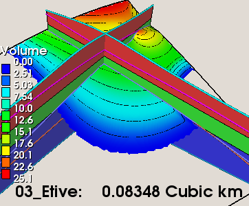
Zone 2 is the Rannoch zone and lays between Rannoch and Etive.
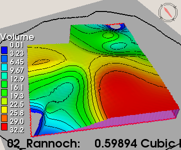
Zone 2 displayed as a single volume isopach
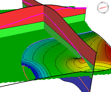
Zone 3 volume map draped on Etive. Cross sections in x and y direction show how Etive goes out of the oil zone and the volume stops. The other layers are shown as lines in the cross sections.
Volume draped on Etive and cross sections at cursor position
The display below shows the volume draped on Etive. The surface above and below and the two contact planes are also displayed. Observe that all volume displays are within the block_area polygon.
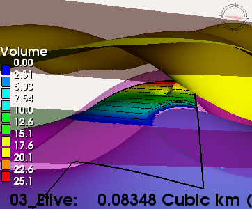
Volume map draped on top horizon of zone 3
An option is to display the surfaces in red green blue colors according to the contact planes. This is shown below for zone 2 with Rannoch as top horizon and Etive as bottom horizon for that zone.
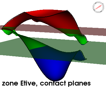
Rannoch zone display between contact planes
A quick way to perform cross sections is to display a fence plot. The layers will be displayed as lines in the cross sections to see their position and zone division.
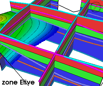
Fence plot with layer lines and volume draped on Etive
To study the layers and the contact planes one can take cross section planes in all three directions. The lines representing the layers in the cross section planes will meet with the same color from the different planes.
Cross section planes in three directions
Tutorial for volume calculation
For further training in volume calculation there is a tutorial at 08 Reservoir and volume calculations. The tutorial utilizes the Course B1 project. Below is a viewport display of the volumetric result through the multilayer reservoir. The generation of the viewport display is explained in the tutorial.
The lower right map shows the contour map of the gas-oil-water contacts. The blue area representing the water zone coincides with the area of no hydrocarbon in the adjacent picture.
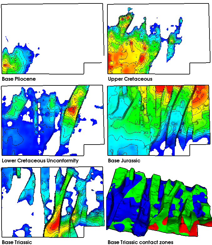
Volume display for all zones in the training project Course B1. The volume map is draped on the top horizon for each zone.
Explanation of the Manipulator page
The manipulator allows a frame to be drawn that will continuously display a cross section of the actual gas-oil-water zones. To use the manipulator a cross section cube has to be generated. Therefore, click on the button Create cross section cube. Then click on Activate and one can draw the cross section plane in all three directions. To display the layers as lines in the cross section plane, click on Make permanent map or Display layers. When leaving the manipulator page, deactivate the manipulator.
The manipulator cube is saved in workspace as cubegrid and may be saved in the project if necessary. If so, it can be placed back into workspace and used as a manipulator cube without generating a new one.
Special features in volume calculation and display.
Calculating volumes for a number of licenses or sub areas.
- Place all the licenses or sub areas i a folder.
- Browse in the folder in the front page.
- Check in Auto report in the Result page.
- Click Execute.
- The execution will be performed for all licenses and sub areas.
- A report is written for each license and sub area.
- When display the results for a particular license, browse in that license and perform Execute over again.
Use the volume menu in a workflow to calculate and display the result.
- Each display option has a check box for automatic display when performing Execute.
- Check in the preferred display and use the menu in a workflow as usual.
Generating a petrophysical grid with a specific fixed value.
Volume calculation using the layer model requires that all petrophysical parameters are grids generated within the same grid window and with the same resolution as the grids in the layer model. When a zone only has a single petrophysical value, that value must be placed in a grid for the matter of consistence. Do as follows:
- any layer_grid > Make Active
- In the command shell: fix value , where value is the petrophysical value.
- Petrophysical folder > New > Workspace Data > active
- Rename active to the proper petrophysical name with the correct prefix (01.., 02.., etc) to have the ordering correct.
Display of contact areas.
- Check in the option: Display contact area (on zone top horizon only).
- Click on Display volume or contact area.
- The contact zones will be contoured as contact areas on the top horizon.
Saving volume reports in the project.
- Go to the Result page.
- Set the save option to disk&folder
- Click on Volume report to:.
- The report is saved to a folder in the project having the same name as the disk report.
- Look at the report by right click > Edit
- You can go back to the graphical window by: toolbar > Window > Geocap