Various types of velocity cubes
Abstract
Stacking velocities are collected along with the seismic surveys. The use of stacking velocities are within depth conversion. One actual transformation of stacking velocities are to model them into a velocity cube. The stacking velocity cube can further be transformed into many variants.
Read about depth conversion in Depth Conversion of time surfaces.
See also the text Creating RMS cube, Interval cube and Depth-Velocity cube.
On this page:
Performing the conversion
The conversion from a time velocity cube to a depth velocity cube is put into the command object Perform calculation on the velocity cube.
Algorithm for generating the depth velocity cube
The following notation is used:
t = time
z = depth
vi = interval velocity
va = average velocity (corrected stacking velocities)
The following formula is applied:
va = z/(t/2000) (time is in millisecond twt)
z = va * t/2000
The result is a z,va cube.
Algorithm for interval velocity cubes
RMS velocity cube:
VRMSn = sqrt((Sum_i(Vi^2*Ti)/Sum_i(Ti))
Interval velocity cube:
IVn = sqrt((VRMSn^2*Tn - VRMSn-1^2*Tn-1)/(Tn-Tn-1))
The result is a time, interval velocity cube.
Menu for calculating various velocity cubes
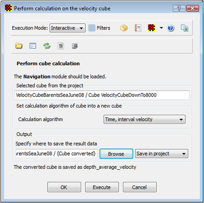
Find the proper action in the combo box and browse in where to save the new velocity cube. Read also the text in the help menu found under ?.
Options for velocity cube calculations
The command object Perform calculation on the velocity cube has an extended list of options. The main part is where the input is a time stacking velocity cube gridded from stacking velocities.
The following cubes can be generated:
- RMS velocity from stacking velocities (SV) -> RMS. Dix formula gives Root Mean Square cube.
- Time, interval velocity, Dix from SV -> RMS -> interval using Dix formula
- Time, average velocity, Dix from SV -> RMS -> interval using Dix formula -> average
- Depth, velocity using probecube A time cube is depth converted using a workspace cube called probecube .
Place the time velocity cube in workspace <b>probecube<b> using the command mhi probecube. - Depth, velocity from SV -> depth_velocity
- Depth, average velocity, Dix from SV -> depth_velocity -> RMS -> interval using Dix formula -> average
- Depth, interval velocity, direct from SV -> depth_velocity -> difference_interval using direct method
- Depth, RMS, interval velocity, Dix from SV -> depth_velocity -> RMS -> interval using Dix formula
- Vertical average sum
Input is any cube and the new cube is just calculated according to the formula.
The following cubes can further be generated:
- Vertical sum , the cells are the sum of the previous cells in the columns.
- Vertical average sum Vertical cells are summed and divided by the distance from the top
- Interval velocity, direct uses vertical velocity interval pairs directly. Use time velocity cube as input
- Interval velocity (Dix) from RMS applies the Dix interval velocity formula on an RMS cube as input
- Time, depth calculates the corresponding depth values in the time plane
- Depth, time calculates the corresponding time values in the depth plane
Various velocity cubes derived from a stacking velocity cube
The picture below shows various calculations of velocity cubes. All cubes have displayed its velocity value at the same xyz position. The z range of the cube is from 0 to 8000 in all cases.
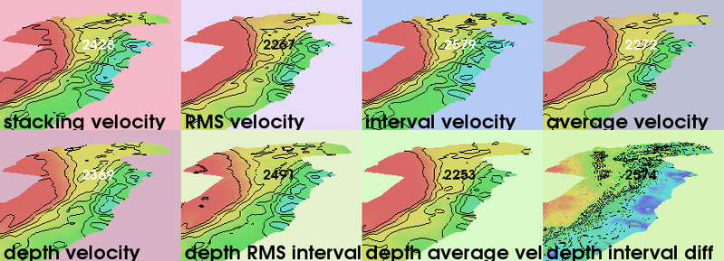
Various velocity cubes derived from a stacking velocity cube
The preferred cube to use in depth conversion is the one that has the most realistic velocity field. Without having some well data for correlation to adjust the stacking velocity cube, that would probably mean to use average velocity which is meant to be the distance traveled divided by the elapsed time.
Example converting a time velocity cube into depth velocity cube
The idea behind a depth velocity map is based on the imagined case that stacking velocities was recording as depth velocity pairs. If that was the case, one could grid up a depth velocity cube the same way as with a time velocity cube.
The task is to first find the corresponding depth value for each time velocity pair. That is done by depth converting the time value. The result depth value is then paired with the same velocity. This is done for all time velocity nodes in the time velocity cube to produce a large set of depth velocity values. These values are then gridded into the depth velocity cube using a vertical interpolation scheme for those grid nodes that have to be filled in.
The result cube is the depth velocity cube and has the same dimensions as the time velocity cube, but the velocity field inside the cube will now follow the depth values in the depth velocity cube. The algorithm corresponds to the formula presented initially.
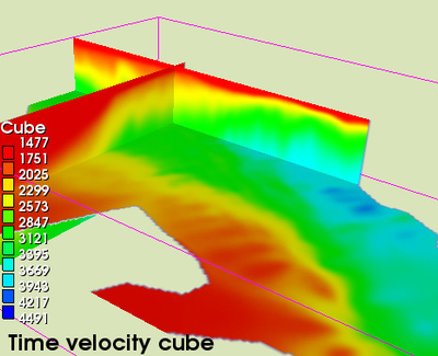
Time velocity cube displayed in three planes
The pictures above shows a standard time velocity cube gridded from stacking velocities. The dimension of the cube is in the time domain, while the contents is the velocity values.
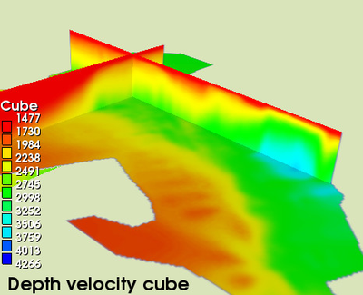
Depth velocity cube displayed in three planes
The picture above shows the depth velocity cube as a result of the conversion algorithm. This cube has the same dimensions as the input cube, but the dimensions of the cube is in the depth domain and the contents is the corresponding velocity values.
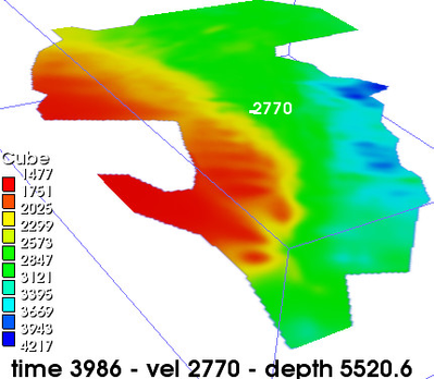
Time velocity cube displayed for time plane 3986
The picture above is from the time-velocity cube and shows the velocity value 2770 for time plane 3986. That correspond to a depth value of 5520.6 units.
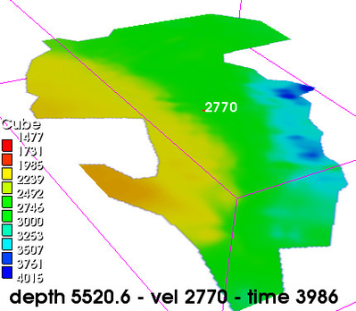
Depth velocity cube displayed for depth plane 5520.6
The picture above is from the depth-velocity cube and shows the velocity value 2770 at the exactly same xy location for depth plane 5520.6. That correspond to a time value of 3986.
The conclusion is that the time and depth cube versus velocity have been inverted.