Generation of time and depth maps in Geocap from 2D seismic
Abstract
This article gives a brief presentation of some work flows in Geocap connected to
interpretation of seismic 2D lines in a heavily faulted area.
Geocap has a unique gridding and modeling capacity that speeds up production time and efficiency towards the final goal:
Converting seismic interpretation into a detailed and accurate mathematical model of the reservoir.
On this page:
Input data
Input data used in this study
- Interpreted seismic lines.
- Interpreted stick faults, i.e. faults without z values.
- RMS stacking velocities.
- Checkshot wells, i.e. drilled wells that show correct depth, time and velocity.
Working procedure in Geocap
The described working procedure in Geocap
- Time grids area created from seismic lines and stick faults.
- A velocity cube was generated from stacking velocities and checkshot wells.
- Depth conversion of time grids to depth grids was performed using the velocity cube.
- Various calculations on the depth grids: volumetric, drainage areas, surface
gradients and extremal values. - High quality Postscript plotting: Geocaps plot module is extremely efficient and
generates a very small Postscript file.
Pictorial series
The following is some pictures and snapshots from a 2D seismic project. The data
have been shifted a little bit from the original. The purpose is to present the
workflows with illustrations.
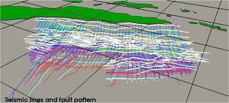
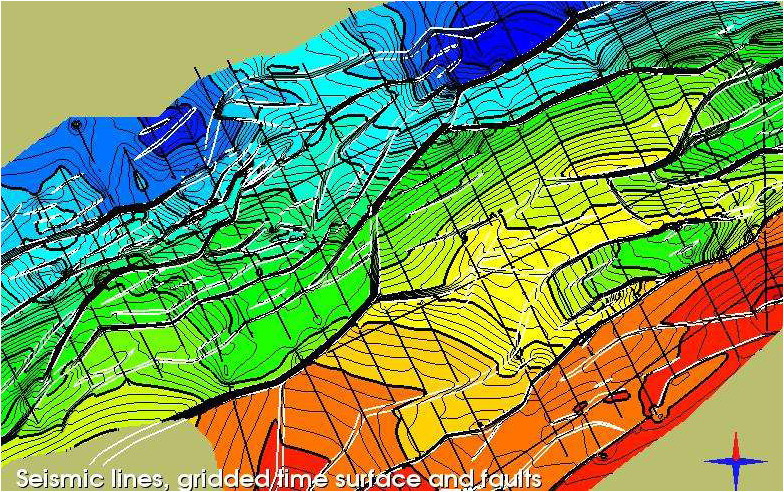
Perspective view of interpreted seismic lines and fault pattern
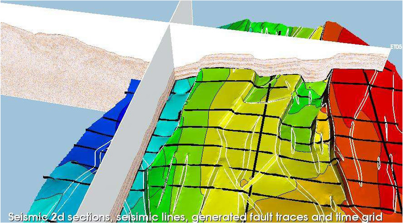
_Seismic 2D sections, interpreted seismic lines for one horizon,
generated fault traces and gridded time surface._
Detail of gridded time surface with interpreted seismic lines.
The faults are generated directly from seismic lines and the fault pattern. The fault
pattern in this case is a set of stick faults without z values. After gridding the
faults will be assigned z values. Geocap has a unique gridding algorithm that takes
as input seismic lines and stick faults, and generates a surface that honors the
faults. This is an automatic and efficient procedure for fast high quality modeling.
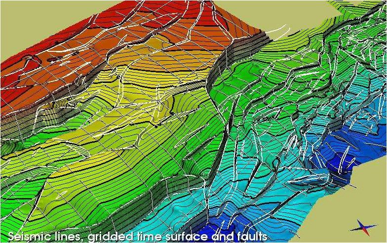
Another detail showing time surface and seismic lines.
Surface overview of fault pattern.
The gridding algorithm can take any number of stick faults, either single fault
lines, or closed stick faults indicating upper and lower part of the faults. In case of
closed fault lines, the algorithm will take lines with or without z values. If without
z values, those fault lines will be assigned z values in the gridding algorithm.
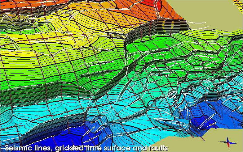
The sophisticated fault logic of the gridding algorithm produces sharp defined
fault transitions in a surface.
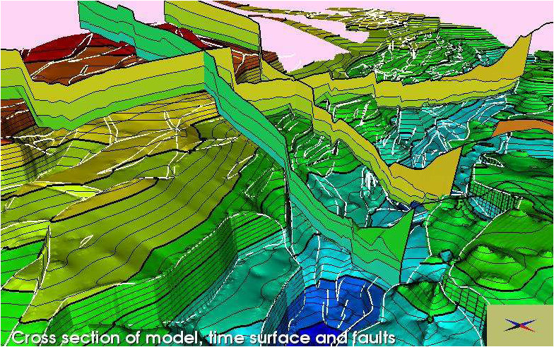
Some cross sections through the time surfaces.
The time surfaces vary a lot with respect to extension and coverage. They are
therefore gridded in separate areas of interest but with same resolution. The cross
section module has no restriction on grid dimensions.
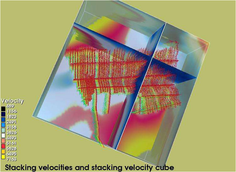
Stacking velocity cube generated from stacking velocities.
A fast and reliable method in Geocap for depth conversion is to generate a
velocity cube from stacking velocities, either RMS velocities or interval velocities
found by Dix formula.
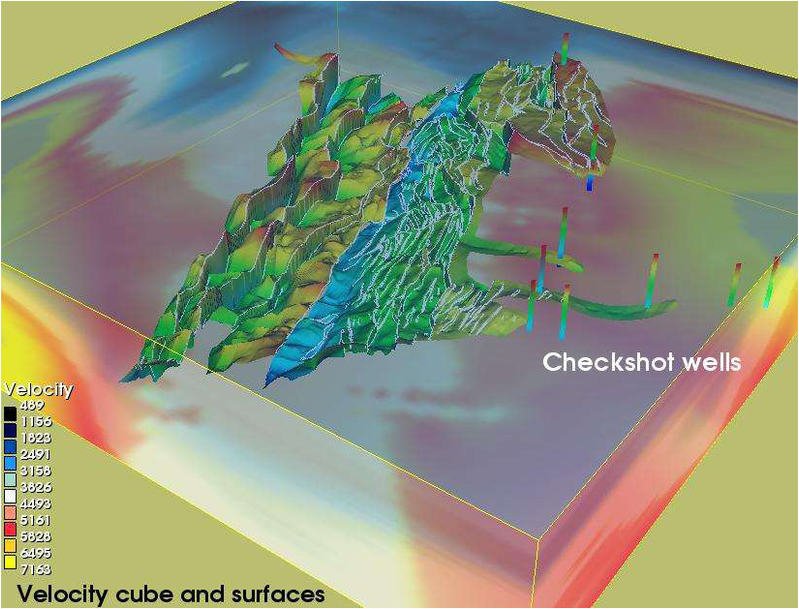
Time surfaces are probed in the velocity cube.
A velocity cube is well suited for depth conversion in a large regional area. The
cube generation process in Geocap will convert the stacking velocities and
checkshot wells into a layered velocity cube model.
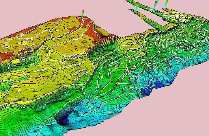
Example of depth grid and fault traces after depth conversion.
Any dataset in time like grids, lines and seismic sections can be depth converted
through the velocity cube. The whole set of time grids and faults traces where
depth converted and controlled that they matched in the checkshot wells.
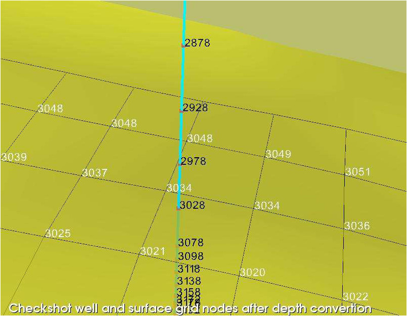
Controlling depth grid and a checkshot well.
Checkshot wells are supposed to be correct and it is always wise to check the
depth conversion in these wells. The velocity cube is correlated with checkshots
in such a way that the conversion should be correct as this display shows.
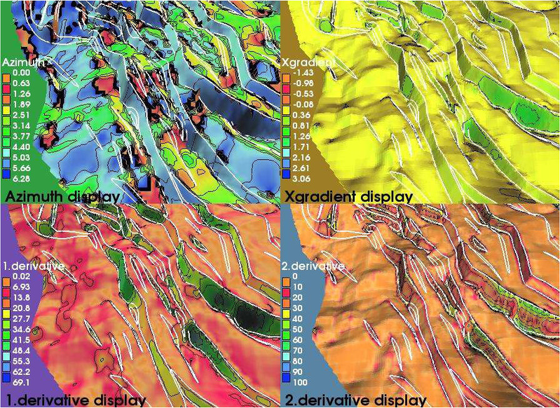
Various attribute maps for a detailed area of a surface.
A user can ask for any kind of attribute map for a surface. Here are just four
examples put together in a view port presentation.
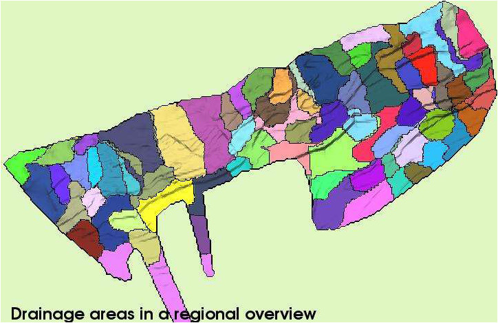
Drainage areas shown in a regional overview presentation.
A drainage area map will tell the specialist about migration and possible prospects
of a reservoir. Geocap has a very good algorithm for such calculations.
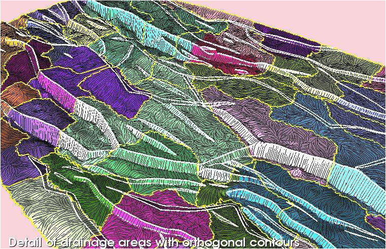
Detailed view of drainage areas with orthogonal contours.
The depth grid can be analyzed for drainage areas using color mapping and
orthogonal contours. A production well should preferably be drilled where the
drainage potential is highest.
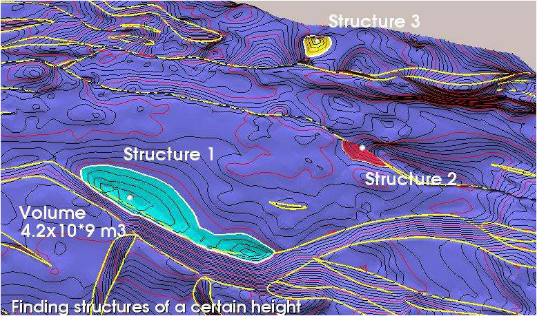
Displaying closed structures of a certain height.
Within prospect analysis Geocap can calculate and map all closed structures of a
certain column height. These are the most obvious candidates for drilling.
Final words
This pictorial set is a brief walk-through of some production workflows in Geocap.
The user operates within a nice interface with a powerful project manager to
control data and command objects. A prolific user can tune the default menus of a
project to preferred settings and options and build up dedicated workflows that fit
the specific project. Working in this fashion and optionally with support from
personnel in Geocap, the user is able to speed up working tasks that are superior
in the oil industry.
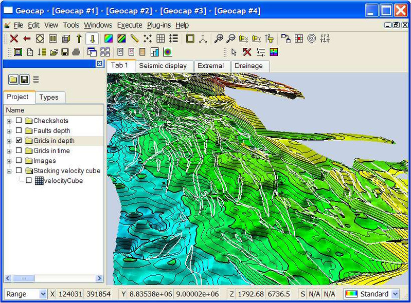
Standard interface of Geocap (previous release)