Time - velocity cube with base grid datum
- Former user (Deleted)
- Erlend Kvinnesland
Introduction
A time-velocity cube (or velocity cube for short) is a set of 2D grids stacked above each other into a 3D cube. The xyz coordinates of the cube is in the time domain while the contents (i.e. the grid nodes) are velocity data. The velocity cube is typically gridded from stacking velocities that consist of vertical lines with x y z velocity information.
The velocity cube is ideal for gridding stacking velocities over flat terrain which means that the cube will have an efficient use of informative grid nodes. The problem occurs when stacking velocities go from shallow water to deep water. Traditionally this would require a large cube to model the whole dataset. The datum of this cube would be MSL (mean sea level) and the content of the cube has water velocity down to the seabed before the interesting velocity values start. To generate a more compact cube one can apply the seabed, or more generally, a base grid as a datum. Then only necessary information will be modeled.
The datum grid or base grid (as it also will be called) can be the seabed, but can also be a little higher up in order to include the transition zone between water and sediments.
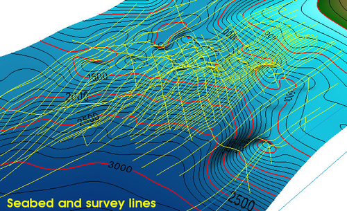
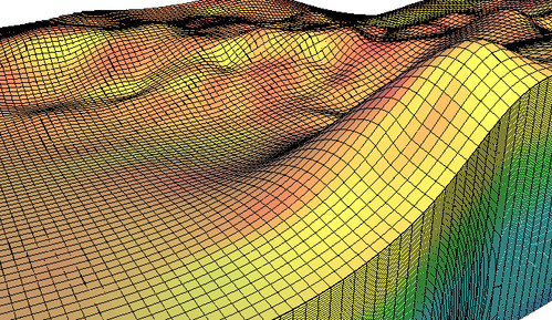
Display of a dipping seabed with seismic survey lines
The base grid datum feature is meant for the experienced user able to use command menus in combination with a few shell commands.
On this page:
Summary of using base grid as datum for stacking velocities and cube
The process of gridding a cube using a base grid as datum involves in principle three steps:
1. Identify the base grid.
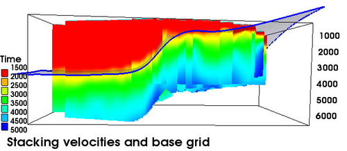
The display below shows stacking velocities and the seabed used as a datum grid.
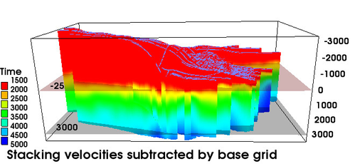
2. Subtract base grid datum from stacking velocities.
All z values in stacking velocities are subtracted the z values of the corresponding positions in the base grid.
The next display shows the result.
3. Grid the time velocity cube.
The interesting information in the datum adjusted stacking velocities are between -25 and 3000 ms which is then used for the cube gridding. The result cube is called base grid cube or just a base cube.
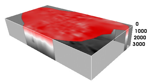
Result base cube with base grid as datum
The base cube in the example has following dimension: x:209 y:106 z:122 = 2702788 nodes == 10558K memory size. The vertical resolution is 25 ms. The corresponding unbased cube would require dimension: x:209 y:106 z:259 = 5737886 nodes == 22414K memory size.
Advantage of a base grid cube
Using a base grid cube across a dipping seabed is efficient in terms of memory space and computer resources.
Creating a base grid
The base grid should preferably be the seabed and can have any resolution. In order to serve as a datum for the cube it must comply with the following requirement:
The extent of the base grid is outside the defined xy area of the cube.
For convenience the base grid is made outside the cube window area, see picture below.
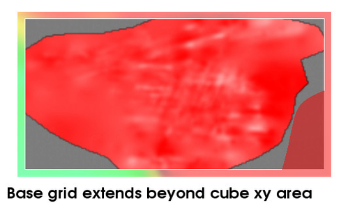
Base grid extents outside cube window
The requirement secures that there is no edge effects when using the base grid as a datum grid towards the cube and stacking velocities and checkshot wells. In a practical situation it is satisfactory that the base grid extents outside the defined area of the cube. If that is not the case one can extend the base grid by regridding it within a closed boundary polygon, or simply apply the command cal xbo (calculate extra border) a few times to create the necessary extra border cells.
For convenience rename the base grid to basegrid and save it in a folder in the project. When using the base grid in algorithms it should also be saved in workspace under the name basegrid.
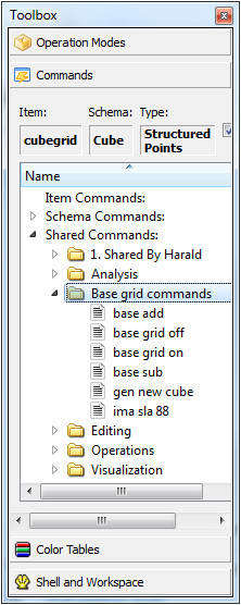
Commands for base grid operations
Handling base grid datum for the velocity cube is done according to the following principles:
- The base grid is placed in workspace basegrid.
- A base grid flag is used to turn on and off the use of the base grid datum.
- Related menus are executed as usual.
A new command called base or just bas has been added to Geocap to handle the base grid operations. The primary syntax is:
base grid commands
base on ; # Probing and selecting cube layers for visualization will use basegrid as a datum.
base off ; # The base grid is turned off as a datum
base new cube ; # Base cube is in active and basegrid is in workspace. Generates a new overall cube cubegrid in workspace. To be used in manipulator display.
base add ; # Data is in active and basegrid is in workspace. Add values in basegrid to the active dataset.
base sub ; # Data is in active and basegrid is in workspace. Subtract values in basegrid to the active dataset.
Creating datasets with basegrid as datum.
For all datasets that should be transformed using the basegrid as datum, the following procedure shall be used:
- Place the base grid in workspace basegrid, i.e copy basegrid from the project and paste it into workspace.
- Make active the dataset to subtract the base grid and perform the command: base sub.
- Save the dataset back into the project.
The procedure above was done for the stacking velocities shown in the display above.
Gridding a base grid cube
When the stacking velocities are datum adjusted by the base grid, the velocity cube can be gridded as normal. One can use the command object Cube gridding from stacking velocities or alternative methods where the layers in the cube are gridded separately and inserted into the cube.
The base cube will have an efficient use of storage with most relevant information filling up the cube.
Visualizing the base cube
The base cube can be visualized in two ways:
- Either as a standard cube with no reference to the base grid.
- If base on is set and basegrid is in workspace, the command object Display selected cube layers will show the correct layer placement and extension. The CO uses the command ima sla 'number' for selecting a certain image layer.
The manipulator visualization of cube data does not test on the base grid flag. The reason for this is that the computing time involved for generating the correct layer from the base cube and the base grid slows down the manipulator so much that it disturbs the manipulator speed. This problem is solved by generating a visualization cube for manipulator display and correct layer display in general.
Generating a visualization cube.
As indicated in the base command reference the syntax for generating a visualization cube is as follows:
The base cube shall be in active and basegrid is in workspace. Execute the command base new cube . Generates a new overall cube cubegrid in workspace. Insert cubegrid into the project and rename it for instance to cubeOverall. This cube has the same number of layers as the base cube and shall be used in the manipulator display. Properties on this cube will show a coarser resolution and is not as appropriate for probing as the denser base cube. But all layers are correct.
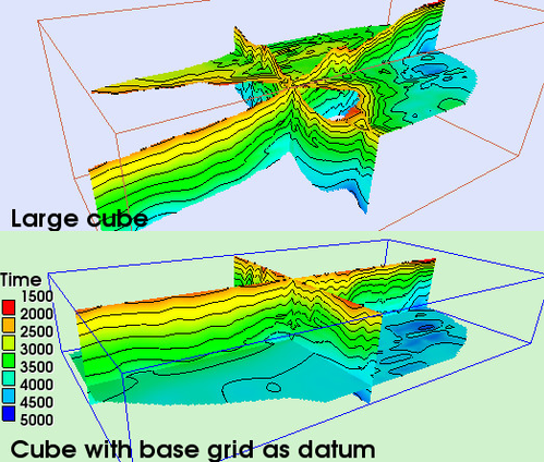
Manipulator used for large cube and base cube
Probing and depth conversion using the base cube
Probing using the base cube can take place as usual for grids, seismic data and datasets in general. All data shall be in there original form. basegrid shall be present in workspace and base on shall be set. Use the standard probing menus which will perform as usual. The probing algorithm will test on the base flag and subtract the base grid to probe in the base cube and add the base grid at the end to get a normal result.
Visualization options
Below is some examples of visualization options with a short explanation.
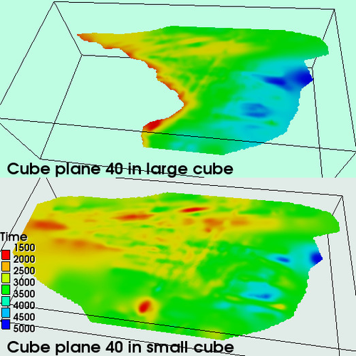
Display of similar layer for large and small cube
The display is performed in a viewport arrangement using the command object Display selected cube layers. To show the large cube one has the option to use the visualization cube directly, or use the base cube with base on and basegrid in workspace.
The smaller cube is the base cube and base off must be active.
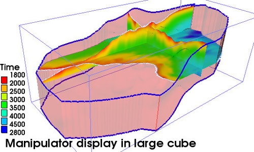
Manipulator display within the cube body
This display used the visualization cube for manipulator display. The body of the cube was generated by making a layer model of the top and bottom surface and displaying the skirt in between; all with low opacity.
To make a top layer: basegrid -> Make Active. fix -25 (if the cube gridding starts from -25). base add. Insert back into the layer model as 01_topgrid.
To make a bottom layer: basegrid -> Make Active. fix 3000 (if the cube gridding ends at 3000). base add. Insert back into the layer model as 05_botgrid.
Use Generate 3d isopachs and skirts to get the skirt.
When the bottom grid is called 05_botgrid it indicates that there could be some grid in between: 02_grid, 03_grid, 04_grid for instance. This was done in the test of the base grid development and depth conversion on the layer model was performed.
Grid cell display of cube body
This display is a cellular display of the cube using an unstructured grid format. It demands more space, but has the flexibility to arrange the cells quite arbitrarily with different spacing and thickness. It parallels pillar grids and general 3D grids. It is created by having a cube in active, then do the command mak uns. Display it by map cel and draw the grid by col bla; poll.
The unstructured grid will not perform well on small computers and should only be used on 64 bits systems. Its intention is for future use if necessary.
Conclusion
This implementation of base grid datum and base cube is technical. The present menus is unchanged. The user must keep in mind the use of base grid and turn it on and off. It is intentionally done that way in order to not disturb the present workflow for generating normal velocity cubes which presumably will still be the standard case until further notice. For the base grid datum cases there should be no problem for an observant user to operate a few commands additionally for applying the base grid. In developing and testing the base grid features a little set in shared commands was made to ease the operation.
Be aware that executing a command from shared commands (or schema commands) will make the activated dataset active; then the command is performed, and then the old active is restored. It is thus necessary to save in workspace the generated result for base add and base sub as shown for the add case:
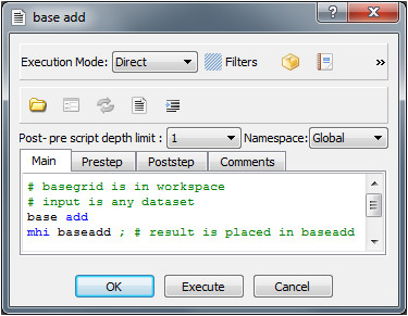
Content of the base add command object
The use of base grid features within the Geocap scripted depth conversion system from Aker Solutions can further be menufied there. This documentation is pure technical and describes the methodology.
Shared command set for base cube manipulation