Layer Model and Cross Sections
- Former user (Deleted)
- Erlend Kvinnesland
Introduction
A folder with ordered surfaces below each other is called a layer model. It has some nice features to be used if there exist two or more surfaces above each other to be placed in the layer model. Then it's easy to perform cross sections and study the layered model through cross section displays.
The purpose of a layer model:
- Overlap and truncation control of all layers
- Generation of 3d isopachs and skirts between layers
- Cross section models and displays
- Generation of cube from layer model
- Depth conversion of grids in a layer model
In this section:
Layer model project
A demo project is established to show the features of the layer model concept. Such a demo project can quickly be generated by anyone following this procedure: (Optionally start a new project first.) Create a Generic folder and apply the command object Demo layer model generation. The folder is renamed to Layer model and the schema type of the folder is set to Layer Model. The name can be a user choice, but the schema of the folder holding the layer model must be Layer Model.
The usual procedure is that a set of grids are placed in a folder. Rename these grids using a prefix 01_.. 02_.. etc so the ordering of the grids are correct according to the sequence from top to bottom. The actual folder with the surface grids in the demo project has been renamed to Horizons 5 layers. The schema type of the folder should be set to Layer Model by applying Horizons 5 layers->Set Schema->Layer Model. The Horizons 5 layers folder now will have command objects visible for layer operations.
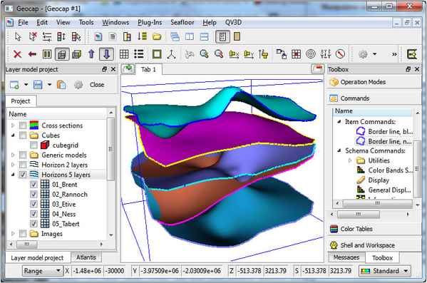
Demo layer model with 5 horizons
Cross sections
One purpose of the layer model is to perform cross sections. To do that one needs a cross section folder to keep the cross section datasets.
Steps to establish and perform cross sections:
- Create a new generic folder and name it Cross sections
- Set the schema to Cross Section
- Apply command Initialize layer model into Workspace
Having established a cross section folder a number of cross section options are available:
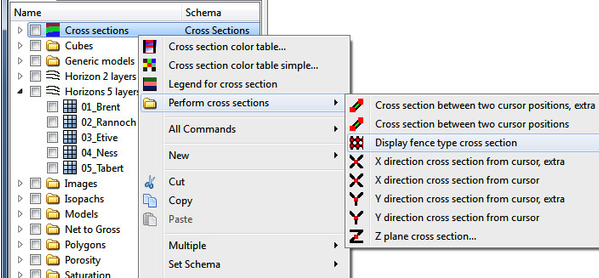
Options in performing cross sections
Example of cross sections on the layer model
The layer model must be initialized by the command layer model->Initialize layer model into Workspace. If one blanks workspace the initialization of the layer model into workspace must be repeated. All the layer grids shall reside in workspace for fast cross section performance.
To display a fence type cross section, do Cross sections->Perform cross sections->Display fence type cross section. One can also add a legend by applying Cross sections->Legend from cross section. The bottom layer is displayed for visualization purpose. The result is shown below.
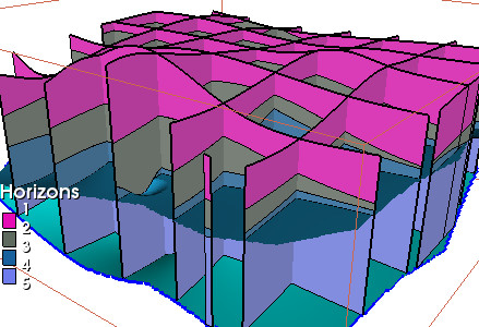
Fence type cross section
Another options is to perform a cross section along a trace (that can go through many wells for instance).
Cross section along a trace:
- Digitize a trace using Quick Digitizing under Tools
- Place the trace in the project and give it a proper name
- Set the schema of the trace to Input Lines To Cross Section
- Apply the command trace > Cross section from line
- The cross section dataset is saved under the trace line
Cross section along a trace
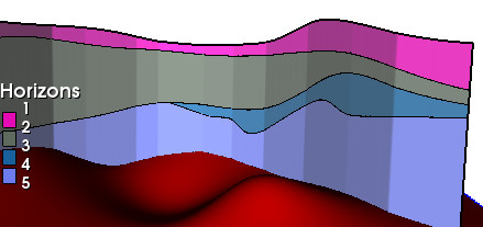
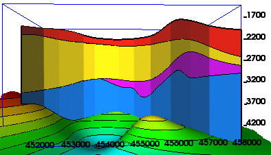
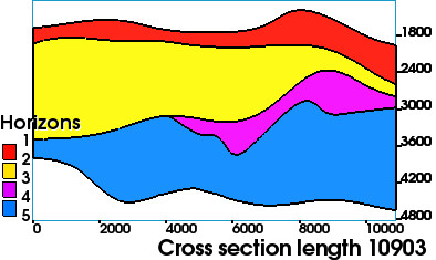
The display below shows various cross section displays. It is possible to make cross sections in all xyz directions.
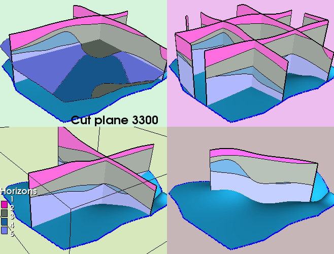
Various cross section through the layer model
The top left viewport display is a cross section for the z plane 3300. The command is Z plane cross section where the z plane value can be set. There is also an option to make the cross section along any arbitrary grid surface.
The top right display is a fence diagram where the number of cross sections are set in the prestep in the command object in edit mode.
The bottom left display is performed using X (and Y) direction cross section from cursor. There are two copies in each direction for practical purposes. If needed, copy and paste the command object to have more options.
The bottom right display is a single cross section between the two last cursor points. Use y to attach the cursor to the surface.
Be sure to follow the guidelines for establishing and using a layer model when horizons are placed in a layer model. Concerning cross sections, the important issue is to initialize the layer model into workspace. That's the rule and using that rule one can shift between various layer models with different number of layers.
Generating layer model cube from the layer model
One purpose with the layer model is to study the geology and layer connections through cross sections. One option for fast cross section studies is to model the layers and the contents in-between into a cube. Then apply the cube manipulator for fast display of cross sections in all three coordinate directions.
Use the command object layer model->Utilities->Cube generation of all layers to model the layers into the cube. The various zones in the layer model get the scalar value according to the number position in the layer model.
The cube should have a reasonable size in order to be held in memory. Prioritize resolution in z direction and the overall size should not exceed 40Mb unless running on a powerful computer.
The cube manipulator is activated by cube->Utilities->Manipulator cube display.
A color table with only four colors was applied for the display. The same color table was activated in the command Cross sections->Cross section color table where the name of the layers can be entered and the cross section legend is displayed.
The named horizons are between the solid zones which have the colors of the color table and shown in the legend.
The bottom horizon called Tarbert is displayed for visual reference.
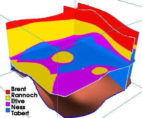
Cube manipulator display applied on a layer cube
Checking overlap and truncation of a layer model
Usually there is a requirement that the interpreted and gridded horizons do not overlap, but instead have eroded surfaces or unconformities. This is handles by the command layer model->Check and truncate layers from top and downwards.
Erotion type between adjacent layers:
- Check and truncate from top
- Check and truncate from bottom
- Half erotion
The help guide in the command says:
This CO is used to secure that a layer model does not overlap. The layers can be given priority from top or from downwards, or the truncation can optionally be divided into equal halves.
A layer in the layer model is checked towards the previous and eroded if overlapping.
All layers are written back into the folder. Therefore, if the original layers are to be kept, make a copy of the layer model first.
If using the operation with Half erosion, after running that feature set truncation option to Check and truncate from top and execute again to get the final truncation towards all layers above.
The intersection option, which is Off by default, is only applied if the defined area of a surface should intersect the next surface to be updated.
It is also possible to be 'creative' and take some layers temporarily out of the layer model using Copy and *Paste to workspace and deleting the same layers in the layer folder. The idea is to let other layers that those in sequence be subjected to mutual truncation. Afterwards add the temporarily saved layers back into the folder.
The check and truncation menu allows for easy trimming of the horizons securing no overlap which means correct volumes and reservoir model.
Generate 3D isopachs and skirts
Having all the horizon layers in a folder it is convenient to generate the isopachs and the skirts between the layers. The isopachs are use in volumetric and reservoir studies. The skirts are mostly used for visualization purposes.
Apply the command layer model->Generate 3d isopachs and skirts and select a proper option to use.
Options for isopach and skirts generation
- Polydata skirt
- Isopach grid
- Isopach polygrid
- 3D grid in space
- Border line
- Layer
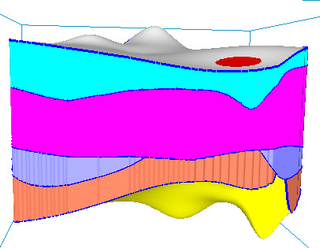
Layer model showing isopachs and skirts
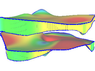
Isopachs generated as 3D grids
Shift layers datum from MSL datum to SRD datum
Definitions
- MSL - mean sea level
- SRD - Seismic Reference Datum
Apply the command layer model > Shift layers datum from MSL to SRD.
This feature is dedicated to cases where the layers are located near the surface and even above MSL. In that case the reservoir model is better handled if all horizons in the layer model are given a new datum higher than the top layer so that all layers have the same sign in their values.
Take a copy of the MSL folder as a backup of a proper MSL set.
Rename the activated folder to a SRD folder.
NB!. This folder must originally be a MSL folder.
The menu will transfer all layer data in the folder to a new datum according to the formula below and the folder will then be a SRD folder.
New datum is transformed according to the shift value.
A positive shift value means that the datum is lifted up the same value.
New horizons: Z(SRD) = shift + sign * Z(MSL)
The use of this menu is actual when the reservoir layers are located above sea level and below sea level, for instance in Wadi areas.
It is then easier to apply standard calculation when all the layers are below a new datum.
Generate layers with constant isopachs and truncate
The purpose of this command object is to quickly establish a layermodel starting with a Truncation surface. The next layers downwards have all constant thickness of varying size. Apply the command layer model->Generate layers with constant isopachs and truncate.
A new layer model is generated from an existing layer model.
In addition one has to select a Start Horizon and a Truncation surface.
The Truncation surface will be the first layer in the new layer model.
All isopachs between the layers are generated with constant thickness specified in the menu for each horizon.
Layer model with two horizons
A layer model with only two horizons can be used for the seabed surface as the bottom horizon and a surface plane at zero value representing the sea level. Then it is easy to perform cross sections all over for visually purposes and also to calculate aera of a cross section as described in the next chapter.
To generate a grid at the sea level, follow this procedure using shell commands:
To generate a grid at sea level:
- seabed_grid > Make Active
- In the shell: fix 0 (all values in the grid are fixed to 0).
- Add the active grid back into the project using New to create a new dataset.
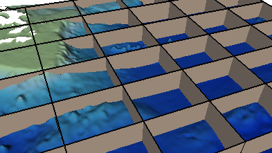
Fence diagram cross section for Atlantis seabed
Area calculation of cross section
Applicable only for cross sections on a layer model with only two horizons. Cross sections can be performed in x and y and arbitrarly directions.
The cross section grid area is found in workspace crossarea.
Procedure for area calculation of a cross section area:
- The layer model must have been initialized into workspace to perform a cross section
- Make one single cross sections through the layer model
- In this case two cursor positions were placed and a cross section from A to B was performed
- The cross section is saved as a dataset
- On the cross section dataset: Use Cross section area calculation
- In this case the result was Calculated area: 5518872064.0
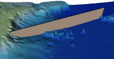
Cross section between two cursor positions
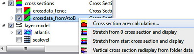
Activating cross section area calculation
Redisplay of cross sections
A cross section dataset will be generated under the cross section folder or cross section trace line when a cross section command is executed. Right click on the cross section dataset the following options appear:
Options for the cross section dataset:
- Cross section area calculation. Mentioned in the chapter above.
- Stretch from 0 cross section and display. Can stretch a curved cross section and redisplay from a zero start position.
- Stretch from start cross section and display. Can stretch a curved cross section and redisplay from the start position.
- Vertical cross section redisplay from folder data. The standard redisplay of a cross section.
When the command Stretch from 0 cross section and display is applied a new tab is created to display the streched cross section. To avoid this if needed, Edit the command and comment the mainwindow statement to #mainwindow newtab "Cross section".
To redisplay properly a color table for the cross sections must be selected. The colors of the cross section are set by the command Cross sections->Cross section color table simpe. Select the appropriate color table and press Execute. For example, prepare a color table with four colors when there are five horizons in the layer model.
A pratical example can be a 30 layer reservoir model where every second layer have hydrocarbons and shall have a certain color. The non hydrocarbon layers shall all have white color. This is easy to set up in a color table and apply in cross section displays.
Cross section along a trace (or through wells)
Stretching out a cross section from zero