F. Basic Concepts in Geocap
- Tore Sannes (Unlicensed)
Introduction
There are a few concepts in Geocap which are important to understand in order to work efficiently with the software. The main concepts are Actors, Schemas, Geodetic Settings and Commands. These concepts will be explained in this section. In addition to this section also talks about toolbars, color tables and keyboard short cuts.
Exercises
Actors
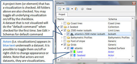
In display context an actor is a graphical term for a visualization unit. A complex display is created by a set of actors. Actors are shown as child's of datasets and are shown in blue text. In Geocap the basic principle is that a display command creates one or several actors. It is possible to remove the actors and the associated display by right clicking and selecting Delete.
Visualizations are called actors
Schemas
By default datasets are organized into data types, such as points and lines (polydata), grids (structured points) etc. These are basic geometric types that contain little information about the domain in which they operate. E.g. coast lines, bathymetric profiles and boundary polygons are all lines (polydata), but the way we work with these types of data are very different and so it is only natural to classify them into different categories. This higher level of classification is made possible by schemas.
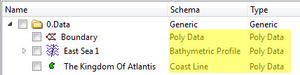
Notice that the dataset types are the same, while the schemas are different
The Geocap modules contains several schemas. For example some of the schemas used in the Shelf Module are coast line, base line, limit line, seabed surface, sediment thickness. You can define the schema of a dataset in the project by right clicking it, and selecting set schema in the pop-up menu. The choice of a dataset´s schema controls which commands you see in the pop-up menu when you right click the dataset. You may create your own schemas as well as edit existing schemas by selecting schemas under edit in the main menu. You can also edit the commands associated with the schemas.
Commands
Commands are operations which can be performed on a dataset. Commands can for example be used to display a dataset in the display window, or to generate new datasets. You can even create your own scripted commands to cater to your specific needs. You execute a command by right clicking the dataset or folder you want to run it on, and then selecting the relevant command in the pop-up menu.
Commands have two execution modes: Direct and Interactive. If the execution mode is set to Interactive the commands editor with the front menu will be displayed when you execute the command. This allows you to adjust various settings that define how the command works. Depending on the command, the menu will consist of different input settings from simple display settings to complex manipulation options. If the execution mode is set to Direct the command will execute with the last active input settings for the command. It is possible to see the underlying settings for any command by right clicking it in the Toolbox and selecting Edit.Note that some commands does not require input parameters and will therefore display the underlying code when running it in Interactive mode.
To see if a command is set to Direct or Interactive mode, look behind the command name. If there are ellipsis (...) behind the name, the command is set to Interactive mode.
All commands have a front end panel, and most of them have settings that may be customized.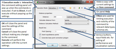
An example of a command front end panel
Commands can be stored in three categories:
- Item commands.
- Schema commands.
- Shared commands.
You will find the commands sorted into the different categories in the Toolbox or on the right-click menu of a dataset or a folder. Commands can also be put together in sequence in Workflows to perform visualizations or data operations.
Item commands
An item command is associated with a single dataset or folder in the project. Item commands are stored along with the project. Therefore, if a project is transferred the item commands will transferred as well. Item commands typically contain settings that pertain specifically to the dataset to which it belongs.
Schema Commands
A schema command is stored with a schema. All datasets or folders using the same schema share these commands, which also means that editing these commands will affect all the datasets using this schema. The schema commands are listed on the right click menu and in the Toolbox under Schema commands.
Get familiar with schema commands
- Right click the different datasets in the project, and see how the right click menu changes from schema to schema.
Tip
The Pin to Menu check box lets you decide which commands should be available in the right click menu, so it is easy to keep organized. Try to experiment with this option to manipulate the right click menu.
Shared Commands
Shared Commands are commands which are shared with all datasets and folders. These commands are always available and listed in the Toolbox under Shared commands.
Default Commands
The default command is the command that is executed when you tick the box next to a dataset in the project. By default a dataset will have one of the schema commands as a default command. This can however be changed to any command.
Change the default display for seabed surfaces
The seabed surfaces has a default command "Map sea" or something similar.
- Click on the Seabed datasets in the Grids folder.
- In the Toolbox right-click another command (i.e LOD Grid Display) and select Set as default command.
- Tick the checkbox next to the Seabed dataset and notice that the new command is executed.
-
Geodetic settings
In Geocap it is the responsibility of the user to secure that data have the correct Datum and Coordinate system, also called a Projection or Geodetic settings. Datasets with the same geographical location but with different coordinate system will not be displayed in the same location in the graphical window. Thus, you will need to convert one of the datasets to the other coordinate system.
View the geodetic settings of a dataset
- Right click any dataset in your project and click Properties.
- Click on the Geodetics tab.
- Observe the Geodetic settings of the dataset.
- Read the warning message.
- Click Close.
You will learn how to convert datasets to other projectons later in this tutorial.
Color Tables
Geocap comes with a set of predefined color tables which can be seen in the toolbox. These color tables are of course customizable, or you can create your own color table from scratch. By default the color tables shown in the lower right corner of Geocap will be used to display a dataset. You can change these color tables by selecting one of them, right-click another color table in the toolbox and select Activate. You can also drag color tables from the toolbox and drop it onto a displayed dataset in the graphical window.
Change the color table on a seabed surface
Visualize a seabed surface.
Click on the Color Tables tab in the Toolbox.
Click, drag and drop one of the color tables on the seabed surface.
Sticky Surface
Geocap has a concept where any surface can be set to be sticky. When a surface is sticky, data like points, lines or images may be displayed onto that surface. This is mainly done by re-sampling lines and displaying them a little bit above the sticky surface. When a surface is activated (or set) as a sticky surface, it is copied to workspace under the name sticky_surface.
Display data on the Sticky Surface
- Right-click on a Seabed surface dataset and select Set as sticky surface.
- Select a line, e.g. Sedimen Data > ATL-99-1 in your project.
- In the Toolbox under Commands > Schema commands right-click Display and click Edit.
- Check the Glue to Sticky Surface and press Execute.
- Investigate the line display.
- Uncheck the Glue to Sticky Surface and press Execute again and observe the difference.
Warning
Note that points and lines displayed onto a sticky surface are displayed without their original z-values, and this may not be what you intend to do when displaying a foot of slope point or a bathymetric line. Keep that in mind.
Toolbar
| Icons | Description of Main Toolbar icons |
|---|---|
| Will cancel any mouse action that is started but is regretted and should be ended without any operation. | |
| Start a mouse action that when clicked on a graphical object will delete that object. | |
| Start a mouse action that when clicked on a graphical object can set appearance parameters for that object. The appearence parameters are: Opacity, Reflection, Diffusion, Ambience. | |
| Start a mouse action where the user is supposed to click on a surface that is map with scalar values. The mapping range of the scalar values according to the color table can then be adjusted. | |
| Start a mouse action that when clicked on a graphical object will highlight the corresponding data object in the project. | |
| Start a mouse action where the user can click and draw a rectangle around displayed data and Geocap will list all dataset names and locations. | |
| Will delete all graphics in the current viewport or window (if the window holds only one viewport). The corresponding references to actors in the project are deleted. Frequently used in free interactive work. | |
| Will delete the last graphical object (also called and actor) that is displayed. Frequently used to erase a graphical object that shall be removed. Note: Redisplaying data from the project using the same command will erase the previous corresponding actor. | |
| Will set the graphical window in 2D mode; i.e. only pan and zoom is allowed. The view direction (x, y or z) depends on the corresponding setting. In 2D mode the left button on the mouse is used for immediate cursor response for instance in digitizing. | |
| Will set the graphical window in 3D mode; pan, zoom and 3D rolling is enabled. The default 3D mode renders in perspective view; i.e. parallel lines are not parallel on the screen, but shows a perspective. | |
| Will turn the z direction of the graphical window upwards; i.e. the positive direction of the z axis points upwards. | |
| Will turn the z direction of the graphical window downwards; i.e. the positive direction of the z axis points downwards. This is the default case because most surfaces are below the zero level, but still have positive z values. | |
| Will show the graphical window as a frame box. It is important to use this icon to check the graphical window or whenever some display comes out weird if the display algorithm uses the graphical window to set display parameters. | |
| Will draw default axes for all visible axes directions. No tick marks are display for simplicity, but the exact location of an annotation position starts at the beginning of the annotation. | |
| Will open a Navigator which is a convenient menu for navigating a 3D graphical scene. To some (especially newbies) it can be difficult to use the mouse buttons to orientate the graphics. Be aware that rotation is around the focal point which also can be set by pointing the cursor mouse at a any location on a solid object and push keyboard x. | |
| Will zoom in towards the focal point. The graphical window is not changed, although the graphical frame may lie out the visible part of the screen. | |
| Will zoom out from the focal point. | |
| Will View from above. This icon also contains sub-icons for viewing in other directions. | |
| If several windows are created on the same Tab, this icon connects the selected windows to the same visual camera. Very useful when different surfaces that shall be compared are displayed in separate windows that are connected and show the same under all graphical movements. | |
| Will show the viewport menu that allows for a quick way to create viewports inside a window. The number and layout of the viewports are determined by just double clicking on the lower right frame in the veiwport menu. If the viewports are connected they can also by used for simultaneously display of surfaces or features that shall be compared. | |
| Enables the light source to be moved around in the graphical scene. Will create shadows and highlight features. Usefull for presentation graphics and detailed studies of special structures. | |
| Will scale the graphical scene with all its actor up or down. Very important for selecting a good view. The scaling should also preferable be set in the Project Settings so that the preferred view comes up when loading a project. | |
| Will show up a 2D compass in upper right that follows the rotation of the graphical window. Another click on the icon will remove the compass. |
Try out the different tools on the toolbar
- Try out the different tools.
-
Keyboard shortcuts
Geocap has several keyboard shortcuts or hotkeys. Go Help > Keyboard shortcuts to bring up a list. A selection of the most important keyboard shortcuts:
| Key | Explanation | Key | Explanation |
|---|---|---|---|
| j | Snap to any point on a displayed line. | + | Zoom in. |
| o | Toggle color code for last used map command on/off. | - | Zoom out. |
| r | Rescale to all graphical elements. | 2 | Toggle graphics to 2d mode. |
| s | Turn graphics into surface mode. | 3 | Toggle graphics to 3d mode. |
| v | Value of height/depth (z coordinate) from graphics. | 3 | Toggle stereo view on/off when stereo is activated. |
| w | Turn graphics into wire mode. | y | Cursor point is set at the surface of the graphical element. |
| x | Setting the focal point. The graphics will rotate around this point. | z | Zoom by drawing a rubber band with left button on the mouse. |
When using j or y to snap to lines or surfaces, Geocap will report what you have snapped to in the lower left corner.
Try the different keyboard shortcuts
- Visualize a seabed surface and test all the above mentioned keyboard shortcuts.